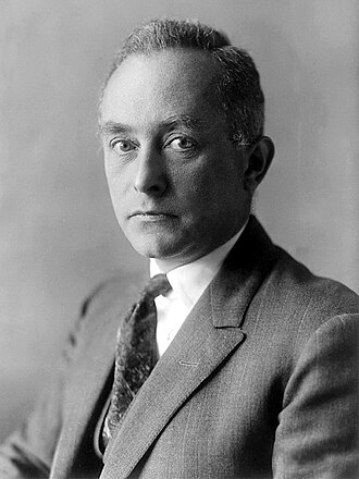
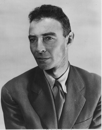
Livro de Texto Universitário Interativo • 6 Blocos • 24 Capítulos Explicados Passo a Passo • 24 Laboratórios • Atlas de 100 Funcionais DFTInteractive University Textbook • 6 Blocks • 24 Step-by-Step Chapters • 24 Laboratories • 100-Entry DFT Functional Atlas
Quantum MechanicsMecânica Quântica
Um manual universitário completo, progressivo e interativo pensado para levar qualquer estudante — mesmo com poucas bases matemáticas iniciais — desde a crise da Física Clássica, postulados quânticos e efeito de túnel 1D até à Superfície de Energia Potencial de Born–Oppenheimer, Hartree–Fock SCF, Conjuntos de Base, Coupled Cluster (CCSD(T)), Teoria do Funcional da Densidade de Kohn–Sham (DFT), Espetroscopia e Termoquímica Computacional.A complete, progressive, interactive university textbook designed to take any student — even with minimal mathematical background — from the crisis of Classical Physics, quantum postulates, and 1D tunnelling all the way to the Born–Oppenheimer Potential Energy Surface, Hartree–Fock SCF, Basis Sets, Coupled Cluster (CCSD(T)), Kohn–Sham Density Functional Theory (DFT), Spectroscopy, and Computational Thermochemistry.
O Que Se Pretende Com o Curso de Mecânica Quântica?What Does the Quantum Mechanics Course Aim to Achieve?
Sempre que uma ligação covalente se quebra ou se forma no centro ativo de uma enzima, sempre que um fotocatalisador absorve luz ou um fármaco reage covalentemente com o seu alvo, os campos de forças clássicos deixam de bastar: entramos no domínio da Mecânica Quântica. Este curso desmistifica a estrutura eletrónica desde os postulados de Schrödinger até aos cálculos modernos de DFT e catálise híbrida QM/MM.Whenever a covalent bond breaks or forms inside an enzyme active site, whenever a photocatalyst absorbs light or a covalent inhibitor reacts with its target, classical force fields are no longer enough: we enter the realm of Quantum Mechanics. This course demystifies electronic structure from Schrödinger's postulates to modern DFT and hybrid QM/MM catalysis.
🌍 Contexto Científico & O Que Se PretendeScientific Context & Course Rationale
Na investigação contemporânea em Química Computacional e Biofísica, programas como o ORCA e o Gaussian são usados diariamente, mas o utilizador corre o risco de escolher funcionais DFT ou conjuntos de base inadequados se não dominar os fundamentos físicos. O nosso objetivo é formar utilizadores críticos, capazes de ligar o formalismo matemático à escolha rigorosa de métodos computacionais.In contemporary Computational Chemistry and Biophysics research, packages like ORCA and Gaussian are used daily, yet practitioners risk choosing flawed DFT functionals or basis sets without solid physical foundations. Our goal is to train critical scientists who connect mathematical formalism to rigorous computational method selection.
✅ Objetivos Principais de AprendizagemCore Learning Objectives
Dominar os Fundamentos e Modelos Exatos (Blocos I–II): Compreender unidades atómicas ($E_h, a_0$), operadores hermíticos, efeito túnel quântico, oscilador harmónico ($ZPE$) e orbitais hidrogenóides 3D.Master Foundations & Exact Models (Blocks I–II): Understand atomic units ($E_h, a_0$), Hermitian operators, quantum tunneling, the harmonic oscillator ($ZPE$), and 3D hydrogenic orbitals.
Compreender Born–Oppenheimer, Hartree–Fock e Conjuntos de Base (Blocos III–IV): Deduzir determinantes de Slater, equações SCF de Roothaan–Hall, STOs vs. CGTOs (def2-TZVP, cc-pVTZ) e erro BSSE.Grasp Born–Oppenheimer, Hartree–Fock & Basis Sets (Blocks III–IV): Derive Slater determinants, Roothaan–Hall SCF equations, STOs vs. CGTOs (def2-TZVP, cc-pVTZ), and BSSE.
Subir a Escada de Jacob da DFT e Correlação Pós-HF (Bloco IV & Cap. 16): Distinguir LDA, GGA, meta-GGA, híbridos e duplos híbridos, dispersão D3(BJ)/D4 e o padrão-ouro $\text{CCSD(T)}$.Climb Jacob's Ladder of DFT & Post-HF Correlation (Block IV & Ch. 16): Distinguish LDA, GGA, meta-GGA, hybrids, double hybrids, D3(BJ)/D4 dispersion, and gold-standard $\text{CCSD(T)}$.
Caracterizar Superfícies de Energia Potencial e Estados de Transição (Blocos V–VI): Localizar mínimos e pontos de sela ($1$ frequência imaginária), seguir caminhos IRC e calcular $\Delta G^\ddagger$ de Eyring.Characterize Potential Energy Surfaces & Transition States (Blocks V–VI): Locate minima and saddle points ($1$ imaginary frequency), trace IRC paths, and compute Eyring $\Delta G^\ddagger$ barriers.
🧭 A Quem Se Destina & Como EstudarWho It Is For & How to Study
Utilize o seletor de profundidade no topo dos capítulos para alternar entre intuição física, deduções matemáticas e comandos práticos (ORCA/Gaussian), explore o Atlas de 100 Funcionais DFT (qm-dft-atlas.html), o Capítulo 16 (Tratado de DFT) (qm-ch16.html) e os 24 Laboratórios Interativos (qm-labs.html).Use the learning-depth switcher to toggle between physical intuition, mathematical derivations, and practical ORCA/Gaussian inputs, and explore the 100-Functional DFT Atlas (qm-dft-atlas.html), Chapter 16 (DFT Treatise) (qm-ch16.html), and the 24 Interactive Labs (qm-labs.html).
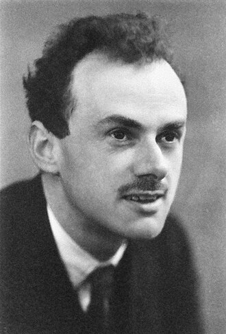
Em 1929, três anos após a descoberta da equação de Schrödinger, Paul Dirac escreveu uma das frases mais célebres da história da ciência: 'As leis físicas subjacentes necessárias para a teoria matemática de grande parte da física e de toda a química são assim completamente conhecidas, e a dificuldade reside apenas no facto de a aplicação exata destas leis conduzir a equações demasiado complexas para serem solúveis.' A história da Mecânica Quântica Molecular é a epopeia de como os físicos e químicos primeiro descobriram essas leis fundamentais (1900–1928) e depois inventaram aproximações físicas geniais — Orbitais Moleculares, Hartree–Fock, Gaussianas, Coupled Cluster e Teoria Funcional da Densidade (DFT) — para tornar essas equações solúveis em moléculas reais.In 1929, Paul Dirac famously declared that the underlying physical laws for all of chemistry were completely known, the only difficulty being that the exact equations were too complex to solve. The history of Quantum Chemistry is the epic story of how physicists and chemists first discovered quantum laws (1900–1928) and then invented brilliant approximations—Molecular Orbitals, Hartree–Fock, Gaussian basis sets, Coupled Cluster, and Density Functional Theory (DFT)—to solve them for real molecules.
0.1 — Era I (1900–1924): A Crise da Física Clássica — Quanta de Planck, Fotões de Einstein, Átomo de Bohr e Ondas de de BroglieEra I (1900–1924): The Crisis of Classical Physics — Planck's Quanta, Einstein's Photons, Bohr's Atom, and de Broglie Waves
0.2 — Era II (1925–1930): A Revolução de Heisenberg, Schrödinger, Born, Pauli e Dirac — O Nascimento da Mecânica OndulatóriaEra II (1925–1930): The Revolution of Heisenberg, Schrödinger, Born, Pauli, and Dirac — Birth of Wave Mechanics
0.3 — Era III (1927–1951): Hartree–Fock, Determinantes de Slater, Ligação de Valência vs. Orbitais Moleculares e HückelEra III (1927–1951): Hartree–Fock, Slater Determinants, Valence Bond vs. Molecular Orbitals, and Hückel Theory
0.4 — Era IV (1952–1985): Simetria Orbital (Fukui & Woodward–Hoffmann) e a Revolução Ab Initio de John PopleEra IV (1952–1985): Orbital Symmetry (Fukui & Woodward–Hoffmann) and John Pople's Ab Initio Revolution
0.5 — Era V (1964–2026): A Revolução da Teoria Funcional da Densidade (DFT), a Escada de Jacob de Perdew, Dispersão D3/D4 e DLPNO-CCSD(T)Era V (1964–2026): The Density Functional Theory (DFT) Revolution, Perdew's Jacob's Ladder, D3/D4 Dispersion, and DLPNO-CCSD(T)
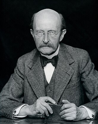
Inaugurou a física quântica em 1900 ao demonstrar que a troca de energia entre matéria e radiação ocorre em pacotes discretos E = h*nu.Inaugurated quantum physics in 1900 by showing that energy exchange between matter and radiation occurs in discrete quanta E = h*nu.
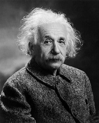
Demonstrou a natureza corpuscular dos quanta de luz (fotões, 1905) e a capacidade calorífica quântica dos sólidos vibracionais (1907).Demonstrated the particle nature of light quanta (photons, 1905) and the quantum heat capacity of vibrating solids (1907).
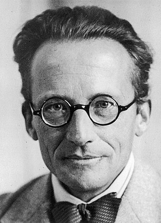
Formulou a mecânica ondulatória em 1926 (H*Psi = E*Psi) e determinou analiticamente as funções próprias e orbitais do átomo de hidrogénio.Formulated wave mechanics in 1926 (H*Psi = E*Psi) and analytically solved the eigenfunctions and orbitals of the hydrogen atom.
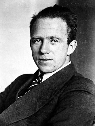
Criou a mecânica matricial de operadores não-comutativos ([x, px] = i*hbar) e o Princípio da Incerteza fundamental.Created matrix mechanics with non-commuting operators ([x, px] = i*hbar) and the fundamental Uncertainty Principle.
Introduziram a função de onda antissimétrica em forma de determinante, as Orbitais Tipo Slater (STOs) e as equações integro-diferenciais de Hartree–Fock.Introduced the determinantal antisymmetric wavefunction, Slater-Type Orbitals (STOs), and the Hartree–Fock equations.
Criaram a teoria das orbitais moleculares deslocalizadas sobre toda a molécula e os diagramas de correlação eletrónica.Created Molecular Orbital theory delocalized over the entire molecule and correlation diagrams.
Demonstrou que a regiosseletividade e as barreiras de ativação química são governadas pela densidade e fase das orbitais de fronteira HOMO e LUMO.Demonstrated that regioselectivity and activation barriers are governed by the density and phase of HOMO and LUMO frontier orbitals.
Formularam as regras de Woodward–Hoffmann para reações pericíclicas, o método de Hückel estendido e a analogia isolobal.Formulated the Woodward–Hoffmann rules for pericyclic reactions, the Extended Hückel method, and the isolobal analogy.
Como Estudar Este Livro de Texto Interativo: Os 6 Blocos Temáticos e os 24 CapítulosHow to Study This Interactive Textbook: The 6 Thematic Blocks & 24 Chapters
Uma progressão pedagógica passo a passo: desde a linguagem matemática elementar até aos cálculos modernos de estrutura eletrónica em moléculas e enzimas.A step-by-step pedagogical progression: from elementary mathematical language to modern electronic structure calculations in molecules and enzymes.
🌍 Bem-Vindo à «Bíblia» Interativa de Mecânica Quântica para Químicos e BioquímicosWelcome to the Interactive Quantum Mechanics "Bible" for Chemists & Biochemists
Se é estudante de Química, Bioquímica, Engenharia Química ou Ciências Farmacêuticas, é muito provável que já se tenha feito esta pergunta: «Porque é que um curso de Química precisa de tanta Mecânica Quântica, e como é que equações com símbolos como \(\hat{H}\Psi = E\Psi\) têm que ver com tubos de ensaio, cores de soluções, fármacos ou enzimas?» A resposta é simples e fascinante: toda a Química é, no seu coração, o resultado das regras da Mecânica Quântica aplicadas aos eletrões. Porque é que o carbono forma quatro ligações tetraédricas e não seis? Porque é que as cenouras são cor de laranja e o sangue arterial é vermelho vivo? Porque é que uma enzima consegue acelerar uma reação um bilião de vezes à temperatura do corpo humano (\(37^\circ\text{C}\))? Nenhuma destas perguntas tem resposta na Física Clássica.If you are a student of Chemistry, Biochemistry, Chemical Engineering, or Pharmaceutical Sciences, you have likely asked yourself: "Why does a Chemistry degree need Quantum Mechanics, and what do equations with symbols like \(\hat{H}\Psi = E\Psi\) have to do with test tubes, solution colors, drugs, or enzymes?" The answer is simple and fascinating: all of Chemistry is, at its heart, the direct consequence of Quantum Mechanics governing electrons. Why does carbon form four tetrahedral bonds rather than six? Why are carrots orange and arterial blood bright red? Why can an enzyme speed up a reaction a trillion-fold at human body temperature (\(37^\circ\text{C}\))? Classical Physics cannot answer a single one of these questions.
Este curso interativo foi desenhado passo a passo com total clareza e rigor pedagógico: nunca se lança uma equação «a frio» sem antes contar a história física, estabelecer um paralelismo com situações familiares do dia a dia e traduzir cada símbolo em linguagem corrente de laboratório. Mesmo que sinta que a sua base matemática está enferrujada, pode ler o texto corrido, as caixas de analogia e os resumos concetuais sem perder o fio condutor — e, quando quiser ver de onde vêm as fórmulas, todas as deduções estão explicadas passo a passo sem saltar etapas.This interactive course was designed step by step for complete pedagogical clarity: it never drops an equation "cold" without first telling the physical story, drawing a parallel to familiar everyday situations, and translating every symbol into plain laboratory language. Even if your mathematical background feels rusty, you can read the narrative prose, analogy boxes, and conceptual summaries without ever losing the thread — and whenever you want to see where a formula comes from, every derivation is explained step by step without skipping a single line.
🗺️ Paralelismo do Mundo Real — Como Navegar Pelos 6 Blocos Como Numa Viagem de Explorador:Real-World Parallel — Navigating the 6 Blocks Like an Explorer's Journey: Imagine que aprender Química Quântica Computacional é como aprender a pilotar um avião moderno ou a tocar um instrumento musical: no Bloco I (Cap. 1–4) aprendemos o alfabeto e as regras básicas do jogo (porque é que os eletrões são ondas); no Bloco II (Cap. 5–8) treinamos em «simuladores de voo simples» com solução exata (uma corda presa nas pontas, uma mola a vibrar, uma bailarina a rodar e o átomo de Hidrogénio isolado); no Bloco III (Cap. 9–12) descobrimos como juntar vários eletrões e vários átomos para formar ligações químicas reais; no Bloco IV (Cap. 13–17) abrimos o motor dos programas modernos (ORCA, Gaussian) para compreender Hartree–Fock, Conjuntos de Base, CCSD(T) e DFT; no Bloco V (Cap. 18–21) usamos esse motor para prever geometrias 3D, estados de transição, espetros IV/RMN e energias livres \(\Delta G^\circ\) em solução; e no Bloco VI (Cap. 22–24) aplicamos tudo a cristais, metais pesados e a um projeto completo de investigação!Imagine learning Computational Quantum Chemistry like learning to fly a modern aircraft or play a musical instrument: in Block I (Ch. 1–4) we learn the alphabet and core rules of the game (why electrons are waves); in Block II (Ch. 5–8) we practice on "simple flight simulators" that can be solved exactly (a guitar string clamped at both ends, a vibrating spring, a spinning skater, and the isolated Hydrogen atom); in Block III (Ch. 9–12) we learn how to bring multiple electrons and nuclei together to form real chemical bonds; in Block IV (Ch. 13–17) we open the hood of modern software packages (ORCA, Gaussian) to master Hartree–Fock, Basis Sets, CCSD(T), and DFT; in Block V (Ch. 18–21) we use that engine to predict 3D geometries, transition states, IR/NMR spectra, and \(\Delta G^\circ\) in solution; and in Block VI (Ch. 22–24) we apply everything to crystals, heavy metals, and a complete research investigation!
⭐ Capítulo em Destaque • Edição Especial ExpandidaFeatured Chapter • Expanded Special Edition
Capítulo 16 — Teoria do Funcional da Densidade (DFT) Explicada Passo a Passo do ZeroChapter 16 — Density Functional Theory (DFT) Explained Step by Step from Scratch
Inclui revisão de base zero (PES, Born–Oppenheimer, notação de Dirac e Unidades Atómicas), Determinante de Slater e Cúspide de Kato, demonstrações comentadas de Hohenberg–Kohn e Levy–Lieb, Equações de Kohn–Sham e Conexão Adiabática (\(\lambda \in [0,1]\)), Buraco de Troca-Correlação \(h_{\text{XC}}\), todos os 5 Degraus da Escada de Jacob, Teorema dos Eletrões Fracionários \(E(N)\) de Perdew–Parr–Levy–Balduz, Dispersão D3(BJ)/D4/VV10, benchmarks reais executados no ORCA 5.0.3 e 8 simuladores interativos!Includes a zero-prerequisite review (PES, Born–Oppenheimer, Dirac notation, and Atomic Units), Slater Determinants and Kato's Cusp, annotated proofs of Hohenberg–Kohn and Levy–Lieb, Kohn–Sham equations and the Adiabatic Connection (\(\lambda \in [0,1]\)), the Exchange-Correlation Hole \(h_{\text{XC}}\), all 5 Rungs of Jacob's Ladder, the Perdew–Parr–Levy–Balduz Fractional-Electron Theorem \(E(N)\), D3(BJ)/D4/VV10 dispersion, real executed ORCA 5.0.3 benchmarks, and 8 interactive simulators!
Índice Interativo dos 24 Capítulos e Registo Pessoal de EstudoInteractive 24-Chapter Index & Personal Study Tracker
📌 Mensagens-Chave — Como Tirar o Máximo Partido Deste ManualKey Takeaways — How to Get the Most Out of This Textbook
A Intuição Física Vem Sempre Primeiro: Antes de olhar para qualquer equação, leia a caixa de contexto e a analogia do quotidiano — se compreender a imagem física (uma corda de guitarra, uma mola, um mapa de trânsito), a fórmula passa a ser apenas uma abreviatura natural dessa ideia.Physical Intuition Always Comes First: Before looking at any equation, read the context box and everyday analogy — once you grasp the physical picture (a guitar string, a spring, a traffic map), the formula becomes merely a shorthand for that idea.
Três Formas de Ler Cada Capítulo: Na 1.ª leitura, pode focar-se no texto principal, nas analogias (💡/🧪), nas dúvidas de estudante (🙋) e nos simuladores interativos (🔬); na 2.ª leitura, explore as caixas azuis de dedução passo a passo (📐) e os problemas resolvidos.Three Ways to Read Every Chapter: On a first reading, focus on the main prose, analogies (💡/🧪), student Q&As (🙋), and interactive simulators (🔬); on a second reading, dive into the step-by-step derivation boxes (📐) and worked problems.
🔗 Ponte para a Secção 01: Onde Começa a Nossa História?Bridge to Section 01: Where Does Our Story Begin?
Agora que conhecemos o mapa dos 6 Blocos e 24 Capítulos, comecemos pela pergunta mais fundamental de todas: porque é que a Física Clássica que aprendemos no ensino secundário falha redondamente quando tentamos descrever um único átomo de Hidrogénio, e qual é a «moeda natural» de energia e distância que os programas de Química Quântica usam no computador?Now that we have seen the map of the 6 Blocks and 24 Chapters, let us start with the most fundamental question of all: why does the Classical Physics we learned in high school fail catastrophically when we try to describe a single Hydrogen atom, and what is the "natural currency" of energy and length used by Quantum Chemistry software on a computer?
01
Capítulo Introdutório I — Porque é que a Mecânica Quântica é Necessária em Química e o Sistema de Unidades Atómicas de Hartree (\(\text{E}_\text{h}, a_0\))Introductory Chapter I — Why Quantum Mechanics Is Needed in Chemistry & Hartree Atomic Units (\(\text{E}_\text{h}, a_0\))
Porque é que os átomos não colapsam, quando é que uma partícula se comporta como onda (\(\lambda = h/p\)) e como ler as energias em Hartree (\(\text{E}_\text{h}\)) impressas pelo ORCA ou Gaussian.Why atoms do not collapse, when a particle behaves as a wave (\(\lambda = h/p\)), and how to read Hartree energies (\(\text{E}_\text{h}\)) printed by ORCA or Gaussian.
🌍 Ponto de Partida Químico: O Mistério da Estabilidade da MatériaChemical Starting Point: The Mystery of Matter's Stability
Olhe para a mão que segura o rato ou para a mesa à sua frente. Ambos são feitos de átomos — um núcleo pequeníssimo e pesado carregado positivamente (protões e neutrões), rodeado por uma nuvem de eletrões levíssimos carregados negativamente. Como cargas opostas se atraem fortemente pela lei de Coulomb, surge imediatamente um enigma que atormentou os físicos e químicos no início do século XX: o que impede os eletrões negativos de caírem imediatamente para cima do núcleo positivo?Look at your hand or the desk in front of you. Both are made of atoms — a tiny, heavy positively charged nucleus (protons and neutrons) surrounded by a cloud of feather-light negatively charged electrons. Because opposite charges attract strongly via Coulomb's law, a puzzle immediately arises that haunted physicists and chemists at the dawn of the 20th century: what stops the negative electrons from crashing straight into the positive nucleus?
Tentou-se primeiro responder que o eletrão girava à volta do núcleo como a Terra gira à volta do Sol. Mas há uma diferença fatal entre um planeta e um eletrão: o eletrão tem carga elétrica! E uma carga elétrica a fazer uma curva funciona exatamente como uma antena de rádio em miniatura: emite ondas eletromagnéticas (luz), perde energia a cada volta e cai em espiral. Compreender como a Natureza evita este desastre é a chave de entrada para toda a Mecânica Quântica.The first attempt was to picture the electron orbiting the nucleus like the Earth orbits the Sun. Yet there is a fatal difference between a planet and an electron: the electron carries electric charge! A charged particle moving along a curved path acts like a miniature radio antenna: it radiates electromagnetic waves (light), loses energy on every turn, and spirals inward. Understanding how Nature prevents this catastrophe is the gateway to all of Quantum Mechanics.
1.1 O Colapso Clássico do Átomo de Rutherford e a Dualidade Onda–Partícula de de Broglie1.1 The Classical Collapse of Rutherford's Atom & de Broglie's Wave–Particle Duality
🙋 Pergunta de Estudante: «Porque é que não podemos simplesmente usar as Leis de Newton (\(\mathbf{F} = m\mathbf{a}\)) para calcular o movimento dos eletrões numa molécula?»Student Question: "Why can't we simply use Newton's Laws (\(\mathbf{F} = m\mathbf{a}\)) to compute the motion of electrons in a molecule?"Resposta clara: Imagine um satélite artificial em órbita baixa à volta da Terra que começa a roçar na atmosfera: ao perder energia por atrito, o satélite perde altitude e acaba por cair na Terra. Na Física Clássica, um eletrão em órbita circular de raio \(r_0 = 0.529\text{ Å}\) em redor de um protão está constantemente a mudar de direção (logo, está acelerado). Pela Eletrodinâmica Clássica de Maxwell, qualquer carga acelerada perde energia emitindo luz continuamente: o eletrão cairia em espiral contra o núcleo em apenas \(\tau_{\text{colapso}} \approx 1.6\times 10^{-11}\text{ s}\) (\(16\) picossegundos)! Nenhum átomo, ligação química ou molécula biológica existiria num universo puramente clássico.Clear answer: Picture an artificial satellite in low Earth orbit experiencing atmospheric drag: as it loses energy, it loses altitude and spirals down to Earth. In Classical Physics, an electron in a circular orbit of radius \(r_0 = 0.529\text{ Å}\) around a proton is constantly changing direction (hence accelerating). By Maxwell's Classical Electrodynamics, any accelerating charge continuously loses energy by radiating light: the electron would spiral into the nucleus in just \(\tau_{\text{collapse}} \approx 1.6\times 10^{-11}\text{ s}\) (\(16\) picoseconds)! No atom, chemical bond, or biological molecule could exist in a purely classical universe.
Como é que a Natureza resolve este paradoxo? Entre 1900 e 1924, Max Planck, Albert Einstein e Louis de Broglie descobriram que os objetos subatómicos não são «pequenos berlindes rígidos». Em vez disso, à escala atómica, a energia é trocada em pacotes discretos (fotões de energia \(\Delta E = h\nu\)) e qualquer partícula em movimento com momento linear \(p = mv\) comporta-se como uma onda no espaço com um comprimento de onda bem definido! O elo de ligação entre o mundo das partículas e o mundo das ondas é a famosa Constante de Planck \(h = 6.62607015\times 10^{-34}\text{ J}\cdot\text{s}\) (ou \(\hbar \equiv \frac{h}{2\pi} = 1.054572\times 10^{-34}\text{ J}\cdot\text{s}\)):How does Nature resolve this paradox? Between 1900 and 1924, Max Planck, Albert Einstein, and Louis de Broglie discovered that subatomic objects are not "tiny hard marbles." Instead, at the atomic scale, energy is exchanged in discrete packets (photons of energy \(\Delta E = h\nu\)) and any moving particle with linear momentum \(p = mv\) behaves as a spatial wave with a well-defined wavelength! The bridge between particles and waves is Planck's Constant \(h = 6.62607015\times 10^{-34}\text{ J}\cdot\text{s}\) (or \(\hbar \equiv \frac{h}{2\pi} = 1.054572\times 10^{-34}\text{ J}\cdot\text{s}\)):
RELAÇÃO DE PLANCK–EINSTEIN E COMPRIMENTO DE ONDA DE DE BROGLIE (1924)PLANCK–EINSTEIN RELATION & DE BROGLIE WAVELENGTH (1924)
$$\Delta E = h\nu = \hbar\omega, \qquad \lambda_{\text{dB}} = \frac{h}{p} = \frac{h}{m v}$$
🎸 Paralelismo com o Dia a Dia — Uma Corda de Guitarra vs. Um Berlinde:Everyday Parallel — A Guitar String vs. A Marble: Porque é que o facto de o eletrão ser uma onda (\(\lambda_{\text{dB}} = h/mv\)) impede o átomo de colapsar? Pense numa corda de guitarra presa nas duas extremidades: pode beliscar a corda para ela vibrar na nota fundamental (\(1\) meia-onda), no 2.º harmónico (\(2\) meias-ondas) ou no 3.º harmónico (\(3\) meias-ondas), mas é fisicamente impossível uma corda presa nas pontas vibrar com \(0.37\) meias-ondas! Da mesma forma, o eletrão preso à volta do núcleo é uma onda estacionária 3D (uma orbital!): ele não pode cair até um raio zero porque uma onda precisa de espaço mínimo para caber sem ter uma energia cinética infinita!Why does the electron's wave nature (\(\lambda_{\text{dB}} = h/mv\)) stop the atom from collapsing? Think of a guitar string clamped at both ends: you can pluck it to vibrate in its fundamental note (\(1\) half-wave), 2nd harmonic (\(2\) half-waves), or 3rd harmonic (\(3\) half-waves), but it is physically impossible for a clamped string to vibrate with \(0.37\) half-waves! Likewise, an electron bound to a nucleus is a 3D standing wave (an orbital!): it cannot collapse to zero radius because a wave requires a minimum volume to fit without acquiring infinite kinetic energy!
🗣️ Tradução em Linguagem Simples — Quando é que a Mecânica Quântica é obrigatória?Plain-Language Translation — When is Quantum Mechanics mandatory? Olhe para a fração \(\lambda_{\text{dB}} = \frac{h}{mv}\): a massa \(m\) está no denominador! Quanto mais leve for a partícula, maior é o seu comprimento de onda \(\lambda_{\text{dB}}\). Compare sempre \(\lambda_{\text{dB}}\) com o tamanho \(d\) da região química (\(\sim 1\text{ a }2\text{ Å}\)):Look at the fraction \(\lambda_{\text{dB}} = \frac{h}{mv}\): the mass \(m\) is in the denominator! The lighter the particle, the larger its wavelength \(\lambda_{\text{dB}}\). Always compare \(\lambda_{\text{dB}}\) with the size \(d\) of the chemical region (\(\sim 1\text{ to }2\text{ Å}\)):
Eletrão num átomo (\(m_e = 9.11\times 10^{-31}\text{ kg}\)): \(\lambda_{\text{dB}} = \mathbf{3.32\text{ Å}}\)! Como a onda do eletrão é maior do que o próprio átomo (\(\sim 1\text{ Å}\)), os eletrões são sempre 100% quânticos!Electron in an atom (\(m_e = 9.11\times 10^{-31}\text{ kg}\)): \(\lambda_{\text{dB}} = \mathbf{3.32\text{ Å}}\)! Because the electron's wave is larger than the atom itself (\(\sim 1\text{ Å}\)), electrons are always 100% quantum mechanical!
Protão \(\text{H}^+\) a \(300\text{ K}\) (\(m_p = 1836\,m_e\)): \(\lambda_{\text{dB}} \approx \mathbf{1.45\text{ Å}}\) — da ordem de uma ligação de hidrogénio! Por isso, a transferência de protões e hidretos em enzimas exibe fortes efeitos quânticos (Energia do Ponto Zero e Efeito de Túnel)!Proton \(\text{H}^+\) at \(300\text{ K}\) (\(m_p = 1836\,m_e\)): \(\lambda_{\text{dB}} \approx \mathbf{1.45\text{ Å}}\) — comparable to a hydrogen bond! Thus proton and hydride transfers in enzymes show strong quantum effects (Zero-Point Energy and Tunnelling)!
Bola de ténis (\(m = 0.058\text{ kg}\)): \(\lambda_{\text{dB}} \approx \mathbf{3.8\times 10^{-34}\text{ m}}\) — biliões de vezes menor que um núcleo! Os efeitos ondulatórios são indetetáveis e a Física Clássica de Newton funciona na perfeição.Tennis ball (\(m = 0.058\text{ kg}\)): \(\lambda_{\text{dB}} \approx \mathbf{3.8\times 10^{-34}\text{ m}}\) — trillions of times smaller than a nucleus! Wave effects are undetectable and Newton's Classical Physics works to perfection.
1.2 A «Moeda Natural» dos Átomos: Unidades Atómicas de Hartree (\(\text{E}_\text{h}, a_0\)) Explicadas Sem Medo1.2 The "Natural Currency" of Atoms: Hartree Atomic Units (\(\text{E}_\text{h}, a_0\)) Explained Without Fear
Se abrir o ficheiro de saída (output) de qualquer programa de Química Quântica moderno — como o ORCA, o Gaussian ou o Psi4 — para uma molécula de água (\(\text{H}_2\text{O}\)), não verá a energia escrita em Joules nem em \(\text{kJ/mol}\), mas sim uma linha como FINAL SINGLE POINT ENERGY = -76.4381245012 Eh. Por que razão os químicos computacionais não usam metros, quilogramas e Joules dentro do computador?If you open the output file of any modern Quantum Chemistry program — such as ORCA, Gaussian, or Psi4 — for a water molecule (\(\text{H}_2\text{O}\)), you will not see the energy printed in Joules or \(\text{kJ/mol}\), but rather a line like FINAL SINGLE POINT ENERGY = -76.4381245012 Eh. Why don't computational chemists use meters, kilograms, and Joules inside the computer?
💶 Paralelismo do Dia a Dia — Porque Não Medimos a Distância entre Coimbra e Lisboa em Milímetros?Everyday Parallel — Why Don't We Measure Highway Distances in Millimeters? No dia a dia, escolhemos sempre unidades adaptadas ao tamanho daquilo que estamos a medir: uma costureira usa centímetros, um automobilista usa quilómetros e um astrónomo usa anos-luz. Medir um eletrão em quilogramas (\(9.11\times 10^{-31}\text{ kg}\)) e metros (\(10^{-10}\text{ m}\)) seria tão absurdo como dizer que a distância de Coimbra a Lisboa é \(200\,000\,000\text{ mm}\)! Em 1928, Douglas Hartree propôs uma ideia genial: usar o próprio átomo de Hidrogénio como régua e balança padrão — definindo a massa de 1 eletrão como \(1\), a carga de 1 eletrão como \(1\), e o raio mais provável do átomo de Hidrogénio como \(1\text{ Bohr}\) (\(a_0 \approx 0.529\text{ Å}\))!In daily life, we always choose units matched to what we are measuring: a tailor uses centimeters, a driver uses kilometers, and an astronomer uses light-years. Measuring an electron in kilograms (\(9.11\times 10^{-31}\text{ kg}\)) and meters (\(10^{-10}\text{ m}\)) would be as awkward as stating a highway distance in millimeters! In 1928, Douglas Hartree proposed a brilliant idea: use the Hydrogen atom itself as the standard ruler and scale — setting the mass of 1 electron to \(1\), the charge of 1 electron to \(1\), and the most probable radius of the Hydrogen atom to \(1\text{ Bohr}\) (\(a_0 \approx 0.529\text{ Å}\))!
📐 Passo a Passo Comentado — Como as Unidades Atómicas Limpam Todas as Constantes da Equação de Schrödinger:Commented Step-by-Step — How Atomic Units Clear All Constants from the Schrödinger Equation:
Em unidades do Sistema Internacional (SI), a Equação de Schrödinger para o eletrão no átomo de Hidrogénio está carregada com quatro constantes físicas (\(m_e, e, \hbar, 4\pi\varepsilon_0\)):In SI units, the Schrödinger Equation for the electron in the Hydrogen atom is cluttered with four physical constants (\(m_e, e, \hbar, 4\pi\varepsilon_0\)):
Em 1928, Douglas Hartree propôs mudar a escala de comprimento para \(\mathbf{r} = a_0\,\mathbf{r}'\) (onde \(\mathbf{r}'\) é medido em múltiplos do raio de Bohr \(a_0\)) e a escala de energia para \(E = \text{E}_\text{h}\,E'\). Substituindo na equação:In 1928, Douglas Hartree proposed rescaling length as \(\mathbf{r} = a_0\,\mathbf{r}'\) (where \(\mathbf{r}'\) is measured in multiples of the Bohr radius \(a_0\)) and energy as \(E = \text{E}_\text{h}\,E'\). Substituting into the equation gives:
Escolhendo \(a_0\) e \(\text{E}_\text{h}\) de modo que os fatores constantes nos dois termos sejam exatamente iguais (\(\frac{\hbar^2}{m_e a_0^2} = \frac{e^2}{4\pi\varepsilon_0 a_0} \equiv \text{E}_\text{h}\)), todas as constantes desaparecem e ficamos com o sistema natural de Unidades Atómicas (\(m_e = e = \hbar = \frac{1}{4\pi\varepsilon_0} = 1\)):By choosing \(a_0\) and \(\text{E}_\text{h}\) so that the prefactors match (\(\frac{\hbar^2}{m_e a_0^2} = \frac{e^2}{4\pi\varepsilon_0 a_0} \equiv \text{E}_\text{h}\)), all constants cancel out, leaving the natural system of Atomic Units (\(m_e = e = \hbar = \frac{1}{4\pi\varepsilon_0} = 1\)):
1.3 Tabela de Conversão de Unidades Quânticas, «Precisão Química» e Simulador Interativo 1.11.3 Quantum Unit Conversion Table, "Chemical Accuracy" & Interactive Simulator 1.1
Um único Hartree (\(\text{E}_\text{h}\)) é uma quantidade colossal de energia à escala de uma reação química à temperatura ambiente: \(1\text{ E}_\text{h} = \mathbf{627.51\text{ kcal/mol}} = \mathbf{2625.5\text{ kJ/mol}}\) — quase o dobro da energia necessária para quebrar uma ligação simples Carbono–Carbono (\(\sim 350\text{ kJ/mol}\))! Por isso, quando comparamos dois isómeros ou calculamos uma barreira de ativação \(\Delta G^\ddagger\) no laboratório, pequenas frações na terceira casa decimal de um Hartree (mili-Hartrees, \(\text{mE}_\text{h}\)) decidem se uma reação ocorre num segundo ou demora anos!A single Hartree (\(\text{E}_\text{h}\)) is a colossal amount of energy on the scale of a room-temperature chemical reaction: \(1\text{ E}_\text{h} = \mathbf{627.51\text{ kcal/mol}} = \mathbf{2625.5\text{ kJ/mol}}\) — nearly twice the energy required to break a Carbon–Carbon single bond (\(\sim 350\text{ kJ/mol}\))! Therefore, when comparing two isomers or computing an activation barrier \(\Delta G^\ddagger\) in the laboratory, tiny fractions in the third decimal place of a Hartree (milli-Hartrees, \(\text{mE}_\text{h}\)) decide whether a reaction takes one second or takes years!
🧪 Paralelismo com o Laboratório Farmacêutico — Porque é que \(1\text{ kcal/mol}\) se chama «Precisão Química»?Pharmaceutical Lab Parallel — Why Is \(1\text{ kcal/mol}\) Called "Chemical Accuracy"?Na Termodinâmica Química (como vimos no curso de TSB!), a constante de equilíbrio \(K_{\text{eq}}\) de um fármaco a ligar-se a uma proteína depende exponencialmente de \(\Delta G^\circ\): \(K_{\text{eq}} = e^{-\Delta G^\circ / RT}\). À temperatura ambiente (\(298.15\text{ K}\)), \(RT \approx 0.592\text{ kcal/mol}\), pelo que mudar \(\Delta G^\circ\) em apenas \(\mathbf{1.364\text{ kcal/mol}}\) (\(\approx 2.17\text{ mE}_\text{h}\)) multiplica ou divide a afinidade do fármaco ou a velocidade da reação por \(10\times\)! Por isso, a comunidade química mundial define \(\mathbf{\pm 1.0\text{ kcal/mol}}\) (\(\approx 1.6\text{ mE}_\text{h}\)) como a meta de «Precisão Química» para qualquer cálculo computacional.In Chemical Thermodynamics (as seen in the TSB course!), the equilibrium constant \(K_{\text{eq}}\) of a drug binding to a protein depends exponentially on \(\Delta G^\circ\): \(K_{\text{eq}} = e^{-\Delta G^\circ / RT}\). At room temperature (\(298.15\text{ K}\)), \(RT \approx 0.592\text{ kcal/mol}\), so shifting \(\Delta G^\circ\) by just \(\mathbf{1.364\text{ kcal/mol}}\) (\(\approx 2.17\text{ mE}_\text{h}\)) multiplies or divides the drug's binding affinity or reaction rate by a factor of \(10\times\)! That is why the global chemistry community defines \(\mathbf{\pm 1.0\text{ kcal/mol}}\) (\(\approx 1.6\text{ mE}_\text{h}\)) as the target of "Chemical Accuracy" for any computational prediction.
Grandeza FísicaPhysical Quantity
Unidade Atómica (Símbolo)Atomic Unit (Symbol)
Equivalência Exata em Unidades ExperimentaisExact Equivalence in Experimental Units
Referência Química MemorávelMemorable Chemical Benchmark
Raio mais provável da orbital \(1s\) do Hidrogénio; ligação \(\text{H–H}\) em \(\text{H}_2\) vale \(1.401\,a_0 = 0.7414\text{ Å}\).Most probable radius of Hydrogen's \(1s\) orbital; \(\text{H–H}\) bond in \(\text{H}_2\) is \(1.401\,a_0 = 0.7414\text{ Å}\).
Energia exata do átomo de Hidrogénio no estado fundamental: \(E_{1s}(\text{H}) = -0.500000\text{ E}_\text{h} = -13.6057\text{ eV}\).Exact ground-state energy of Hydrogen atom: \(E_{1s}(\text{H}) = -0.500000\text{ E}_\text{h} = -13.6057\text{ eV}\).
A \(298.15\text{ K}\), um erro de \(1.364\text{ kcal/mol}\) altera uma constante de equilíbrio \(K_{\text{eq}}\) num fator de \(10\times\)!At \(298.15\text{ K}\), an error of \(1.364\text{ kcal/mol}\) shifts an equilibrium constant \(K_{\text{eq}}\) by a factor of \(10\times\)!
Um eletrão completa uma «órbita de Bohr» em \(2\pi\tau_0 \approx 152\text{ as}\), enquanto uma vibração \(\text{O–H}\) demora \(\sim 10\text{ fs}\)!An electron completes a "Bohr orbit" in \(2\pi\tau_0 \approx 152\text{ as}\), whereas an \(\text{O–H}\) vibration takes \(\sim 10\text{ fs}\)!
🔬 Interativo 1.1Interactive 1.1Conversor de Energia Quântica e Impacto Termodinâmico em \(K_{\text{eq}}\) (\(298.15\text{ K}\))Quantum Energy Converter & Thermodynamic Impact on \(K_{\text{eq}}\) (\(298.15\text{ K}\))
🎯O Que Se Pretende Fazer Neste Simulador e PorquêWhat This Simulator Does & Why It Matters
Objetivo: Ganhar intuição imediata para as unidades dos programas quânticos (Hartree \(\text{E}_\text{h}\), Bohr \(a_0\), \(\text{kcal/mol}\), \(\text{kJ/mol}\) e \(\text{eV}\)) e compreender porque é que um erro aparentemente minúsculo de \(0.0022\text{ E}_\text{h}\) (\(1.36\text{ kcal/mol}\)) altera uma constante de equilíbrio \(K_{\text{eq}}\) ou a potência de um fármaco em \(10\times\) à temperatura ambiente. Use o seletor ou o cursor e clique em ℹ️ Explicação deste seletor abaixo de cada controlo para ver o que fazer.Goal: Build instant intuition for quantum software units (Hartree \(\text{E}_\text{h}\), Bohr \(a_0\), \(\text{kcal/mol}\), \(\text{kJ/mol}\), and \(\text{eV}\)) and see why a seemingly tiny \(0.0022\text{ E}_\text{h}\) (\(1.36\text{ kcal/mol}\)) error changes an equilibrium constant \(K_{\text{eq}}\) or drug binding affinity by \(10\times\) at room temperature. Adjust the controls or click ℹ️ Control explanation below each selector.
ℹ️ Explicação deste seletor / controlo (clique para abrir)ℹ️ Explanation of this selector / control (click to open)
O que controla: Define a diferença de energia (ou erro de cálculo) \(\Delta E\) em \(\text{kcal/mol}\). Porquê experimentar: Permite ver instantaneamente a conversão para Hartree (\(\text{E}_\text{h}\)), milihartree (\(\text{mE}_\text{h}\)), \(\text{kJ/mol}\) e \(\text{eV}\), e sobretudo como um pequeno erro energético se amplifica exponencialmente na razão de constantes de equilíbrio \(K_2/K_1 = e^{\Delta E/RT}\) a \(298.15\text{ K}\).What it controls: Sets the energy difference (or computational error) \(\Delta E\) in \(\text{kcal/mol}\). Why experiment with it: Shows the instant conversion into Hartree (\(\text{E}_\text{h}\)), millihartree (\(\text{mE}_\text{h}\)), \(\text{kJ/mol}\), and \(\text{eV}\), and demonstrates how a small energy error amplifies exponentially in the equilibrium ratio \(K_2/K_1 = e^{\Delta E/RT}\) at \(298.15\text{ K}\).
ℹ️ Explicação deste seletor / controlo (clique para abrir)ℹ️ Explanation of this selector / control (click to open)
O que faz este seletor: Carrega automaticamente valores de referência reais da Química e da Bioquímica (energia térmica \(RT\), fasquia de «Precisão Química» de \(1.0\text{ kcal/mol}\), erro de \(1.36\text{ kcal/mol}\) que altera \(K_{\text{eq}}\) em \(10\times\), barreira de rotação do etano ou ponte de hidrogénio na água).What this selector does: Automatically loads real chemical and biochemical benchmarks (thermal energy \(RT\), the \(1.0\text{ kcal/mol}\) "Chemical Accuracy" target, the \(1.36\text{ kcal/mol}\) shift that changes \(K_{\text{eq}}\) by \(10\times\), ethane's rotation barrier, or a water hydrogen bond).
Número de Onda (\(\text{cm}^{-1}\))Wavenumber (\(\text{cm}^{-1}\))
349.8 cm⁻¹
Fator em \(K_{\text{eq}}\) (\(298\text{ K}\))Factor in \(K_{\text{eq}}\) (\(298\text{ K}\))
5.4×
📌 Mensagens-Chave para o Químico — Capítulo Introdutório IKey Takeaways for Chemists — Introductory Chapter I
Os eletrões são ondas estacionárias 3D (orbitais): Porque o comprimento de onda de de Broglie do eletrão (\(\lambda_{\text{dB}} \approx 3.3\text{ Å}\)) é da ordem do tamanho do próprio átomo, a Mecânica Quântica é indispensável para descrever qualquer ligação química.Electrons are 3D standing waves (orbitals): Because the electron's de Broglie wavelength (\(\lambda_{\text{dB}} \approx 3.3\text{ Å}\)) matches the size of the atom itself, Quantum Mechanics is indispensable for describing any chemical bond.
Unidades Atómicas (\(\text{E}_\text{h}, a_0\)): Todos os programas quânticos trabalham na «moeda natural do átomo de Hidrogénio» (\(1\,a_0 = 0.529\text{ Å}\) e \(1\text{ E}_\text{h} = 627.51\text{ kcal/mol} = 2625.5\text{ kJ/mol}\)). Atingir a «Precisão Química» (\(\pm 1\text{ kcal/mol}\)) exige acertar nas diferenças de energia até \(0.0016\text{ E}_\text{h}\)!Atomic Units (\(\text{E}_\text{h}, a_0\)): All quantum packages compute in the "natural currency of the Hydrogen atom" (\(1\,a_0 = 0.529\text{ Å}\) and \(1\text{ E}_\text{h} = 627.51\text{ kcal/mol} = 2625.5\text{ kJ/mol}\)). Achieving "Chemical Accuracy" (\(\pm 1\text{ kcal/mol}\)) requires resolving energy differences to \(0.0016\text{ E}_\text{h}\)!
🔗 Ponte para a Secção 02: Como Resolver a Equação de Schrödinger para Moléculas Reais?Bridge to Section 02: How Do We Solve the Schrödinger Equation for Real Molecules?
No átomo de Hidrogénio (\(1\) único eletrão), a Equação de Schrödinger resolve-se exatamente no papel. Mas o que acontece quando passamos para o benzeno (\(42\) eletrões), a cafeína (\(102\) eletrões) ou uma enzima? Na Secção 02 vamos conhecer o mapa das duas grandes famílias de métodos que permitem aos químicos resolver moléculas reais!In the Hydrogen atom (just \(1\) electron), the Schrödinger Equation can be solved exactly with pen and paper. But what happens when we move to benzene (\(42\) electrons), caffeine (\(102\) electrons), or an enzyme? In Section 02 we explore the master map of the two great method families that allow chemists to solve real molecules!
02
Mapa Geral da Química Quântica Computacional: Como se Ligam Todos os Métodos dos 24 Capítulos?Master Map of Computational Quantum Chemistry: How Do All Methods Across the 24 Chapters Connect?
Uma visão panorâmica das duas grandes estradas para resolver a Equação de Schrödinger Eletrónica: a Escada da Função de Onda (\(\Psi\)) vs. a Escada da Densidade Eletrónica (\(\rho(\mathbf{r})\), DFT).A panoramic view of the two great highways for solving the Electronic Schrödinger Equation: the Wavefunction Ladder (\(\Psi\)) vs. the Electron Density Ladder (\(\rho(\mathbf{r})\), DFT).
🌍 Ponto de Partida Químico: O «Menu de Siglas» dos Programas de Química ComputacionalChemical Starting Point: The "Acronym Menu" of Computational Chemistry Software
Quando um estudante abre um artigo científico ou o manual do ORCA / Gaussian, depara-se com dezenas de siglas misteriosas: RHF, MP2, CCSD(T), B3LYP, PBE0, r2SCAN-3c, ωB97M-V, CASSCF. Porque é que existem tantos métodos em vez de um só? A razão é o chamado problema dos muitos corpos: numa molécula com \(N\) eletrões, todos os eletrões se repelem mutuamente ao mesmo tempo, desviando-se uns dos outros a cada instante. Como não existe solução analítica exata para \(N \ge 2\) eletrões, os químicos criaram duas estradas inteligentes para aproximar essa dança coletiva dos eletrões!When a student opens a research paper or the ORCA / Gaussian manual, they face dozens of mysterious acronyms: RHF, MP2, CCSD(T), B3LYP, PBE0, r2SCAN-3c, ωB97M-V, CASSCF. Why do so many methods exist instead of just one? The reason is the many-body problem: in a molecule with \(N\) electrons, all electrons repel each other simultaneously, swerving around one another at every instant. Because no exact analytical solution exists for \(N \ge 2\) electrons, chemists built two clever highways to approximate this collective electron dance!
2.1 As Duas Grandes Famílias de Métodos: Métodos Baseados na Função de Onda (\(\Psi\)) vs. DFT de Kohn–Sham (\(\rho(\mathbf{r})\))2.1 The Two Great Method Families: Wavefunction-Based Methods (\(\Psi\)) vs. Kohn–Sham DFT (\(\rho(\mathbf{r})\))
🚗 Paralelismo com o Dia a Dia — Seguir o Diário de Viagem de Cada Condutor (\(\Psi\)) vs. Olhar para o Mapa de Trânsito por Satélite (\(\rho(\mathbf{r})\)):Everyday Parallel — Tracking Every Driver's Travel Diary (\(\Psi\)) vs. Viewing a Satellite Traffic Density Map (\(\rho(\mathbf{r})\)): Imagine que quer calcular o trânsito numa cidade com \(100\) automóveis (os nossos \(100\) eletrões):
• Na Estrada A (Métodos de Função de Onda \(\Psi\): HF \(\to\) MP2 \(\to\) CCSD(T)), começamos por assumir que cada condutor guia apenas olhando para a média habitual do trânsito (Hartree–Fock), e depois calculamos explicitamente como cada par ou trio de carros se desvia em tempo real nos cruzamentos (MP2 e CCSD(T)). É extremamente rigoroso, mas o esforço de cálculo explode rapidamente (\(\mathcal{O}(N^7)\)) quando o número de carros aumenta!
• Na Estrada B (Teoria do Funcional da Densidade, DFT), Walter Kohn mostrou que não precisamos de seguir cada par de carros individualmente: basta conhecer o mapa 3D da densidade de trânsito \(\rho(x,y,z)\) em cada rua da cidade! Isso permite estudar moléculas com \(100\text{ a }1\,000\) átomos numa fração do tempo!Imagine you want to model traffic in a city with \(100\) cars (our \(100\) electrons):
• On Highway A (Wavefunction Methods \(\Psi\): HF \(\to\) MP2 \(\to\) CCSD(T)), we start by assuming each driver reacts only to the average daily traffic map (Hartree–Fock), and then explicitly compute how every pair and trio of cars swerves around each other at intersections (MP2 and CCSD(T)). It is extraordinarily accurate, but the computer cost explodes (\(\mathcal{O}(N^7)\)) as the number of cars grows!
• On Highway B (Density Functional Theory, DFT), Walter Kohn proved we do not need to track every simultaneous pair of cars: knowing the 3D traffic density map \(\rho(x,y,z)\) on each street suffices! This lets us study molecules of \(100\text{ to }1,000\) atoms in a fraction of the time!
Quase todos os cálculos que um químico computacional executa partem da Equação de Schrödinger Eletrónica na Aproximação de Born–Oppenheimer (Capítulos 11 a 17): fixamos os núcleos nas posições \(\mathbf{R}_A\) e procuramos a energia dos \(N\) eletrões, \(E_{\text{el}}(\mathbf{R})\). Como o termo de repulsão intereletrónica \(\sum_{i\lt j}\frac{1}{r_{ij}}\) acopla o movimento de todos os eletrões, a Química Quântica desenvolveu estas duas grandes estratégias complementares:Nearly all calculations performed by a computational chemist start from the Electronic Schrödinger Equation within the Born–Oppenheimer Approximation (Chapters 11 to 17): we clamp the nuclei at positions \(\mathbf{R}_A\) and solve for the energy of the \(N\) electrons, \(E_{\text{el}}(\mathbf{R})\). Because the electron–electron repulsion \(\sum_{i\lt j}\frac{1}{r_{ij}}\) couples all electrons together, Quantum Chemistry developed these two complementary strategies:
Estrada A: Hierarquia Ab Initio de Função de Onda (\(\Psi\))Highway A: Ab Initio Wavefunction Hierarchy (\(\Psi\))
Capítulos 13, 14, 15 e 17 (Bloco IV): Começa num único Determinante de Slater (Hartree–Fock, \(\text{HF}\), que trata a repulsão de Coulomb como um campo médio e inclui \(100\%\) da troca exata de Pauli, mas \(0\%\) de correlação eletrónica). Depois adiciona sistematicamente excitações eletrónicas para orbitais virtuais: \(\text{MP2}\) \(\mathcal{O}(N^5) \to\) \(\text{CCSD}\) \(\mathcal{O}(N^6) \to\) \(\text{CCSD(T)}\) \(\mathcal{O}(N^7)\) («Padrão de Ouro») \(\to\) \(\text{Full CI}\) \(\mathcal{O}(N!)\).Chapters 13, 14, 15 & 17 (Block IV): Starts from a single Slater Determinant (Hartree–Fock, \(\text{HF}\), which treats Coulomb repulsion as a mean field and includes \(100\%\) exact Pauli exchange, but \(0\%\) electron correlation). It then systematically adds virtual orbital excitations: \(\text{MP2}\) \(\mathcal{O}(N^5) \to\) \(\text{CCSD}\) \(\mathcal{O}(N^6) \to\) \(\text{CCSD(T)}\) \(\mathcal{O}(N^7)\) ("Gold Standard") \(\to\) \(\text{Full CI}\) \(\mathcal{O}(N!)\).
Estrada B: Teoria do Funcional da Densidade (\(\rho(\mathbf{r})\), DFT)Highway B: Density Functional Theory (\(\rho(\mathbf{r})\), DFT)
Capítulo 16 (Edição Completa DFT e Atlas de 100 Funcionais): Em vez da função de onda de \(3N\) coordenadas, calcula a energia a partir da densidade eletrónica 3D \(\rho(x,y,z)\) usando \(N\) orbitais de Kohn–Sham para obter a energia cinética exata \(T_s\) e englobando a troca e a correlação no funcional \(E_{\text{XC}}[\rho]\) ao longo dos 5 degraus da Escada de Jacob, mantendo um custo muito baixo \(\mathcal{O}(N^3\text{–}N^4)\)!Chapter 16 (Full DFT Textbook & 100-Functional Atlas): Instead of the \(3N\)-coordinate wavefunction, it computes the energy from the 3D electron density \(\rho(x,y,z)\) using \(N\) Kohn–Sham orbitals for the exact non-interacting kinetic energy \(T_s\) and folding exchange and correlation into \(E_{\text{XC}}[\rho]\) across the 5 rungs of Jacob's Ladder at low \(\mathcal{O}(N^3\text{–}N^4)\) cost!
2.2 Tabela Comparativa de Métodos de Estrutura Eletrónica: Precisão, Escalabilidade e Quando Escolher2.2 Electronic Structure Method Comparison Table: Accuracy, Scaling & When to Choose
Na coluna «Escalonamento» da tabela abaixo encontrará expressões como \(\mathcal{O}(N^3)\) ou \(\mathcal{O}(N^7)\). O que significa isto na prática quando está à espera que o computador termine um cálculo? Se duplicar o tamanho da sua molécula (\(2\times\) mais átomos/eletrões), um método \(\mathcal{O}(N^3)\) demora \(2^3 = \mathbf{8\times}\) mais tempo (por exemplo, passa de \(1\text{ minuto}\) para \(8\text{ minutos}\)); já um método \(\mathcal{O}(N^7)\) como o CCSD(T) canónico demora \(2^7 = \mathbf{128\times}\) mais tempo (passa de \(1\text{ hora}\) para \(5\text{ dias}\))!In the "Scaling" column of the table below you will see expressions such as \(\mathcal{O}(N^3)\) or \(\mathcal{O}(N^7)\). What does this mean in practice when waiting for your computer calculation to finish? If you double the size of your molecule (\(2\times\) more atoms/electrons), an \(\mathcal{O}(N^3)\) method takes \(2^3 = \mathbf{8\times}\) longer (e.g., from \(1\text{ minute}\) to \(8\text{ minutes}\)), whereas a canonical \(\mathcal{O}(N^7)\) method like CCSD(T) takes \(2^7 = \mathbf{128\times}\) longer (from \(1\text{ hour}\) to \(5\text{ days}\))!
\(\sim 10\text{ a }30\text{ kcal/mol}\) (sem correlação!)\(\sim 10\text{ to }30\text{ kcal/mol}\) (no correlation!)
Ponto de partida para métodos pós-HF (MP2, CCSD(T)); ensino do ciclo SCF e troca exata.Starting point for post-HF methods (MP2, CCSD(T)); teaching SCF and exact exchange.
\(\sim 2.5\text{ a }5.0\text{ kcal/mol}\)\(\sim 2.5\text{ to }5.0\text{ kcal/mol}\)
Otimização rápida de geometrias, frequências vibracionais e sistemas periódicos/grandes (\(>200\) átomos).Fast geometry optimizations, vibrational frequencies, and large/periodic systems (\(>200\) atoms).
\(\mathbf{\sim 1.5\text{ a }2.8\text{ kcal/mol}}\)\(\mathbf{\sim 1.5\text{ to }2.8\text{ kcal/mol}}\)
O cavalo de batalha universal para reatividade orgânica, bioinorgânica, catálise e estados excitados TDDFT.Universal workhorse for organic, bioinorganic, catalytic reactivity, and TDDFT excited states.
\(\mathbf{\sim 1.2\text{ a }1.8\text{ kcal/mol}}\)\(\mathbf{\sim 1.2\text{ to }1.8\text{ kcal/mol}}\)
Energias single-point de alta precisão em moléculas do grupo principal sem forte caráter multirreferência.High-accuracy single-point energies in main-group molecules without strong multireference character.
\(\mathbf{\le 0.5\text{ a }1.0\text{ kcal/mol}}\) («Precisão Química»!)\(\mathbf{\le 0.5\text{ to }1.0\text{ kcal/mol}}\) ("Chemical Accuracy"!)
Referência «Padrão de Ouro» para energias de reação e barreiras de sistemas bem descritos por 1 referência (\(T_1 \lt 0.02\))."Gold Standard" reference for reaction energies and barriers of single-reference systems (\(T_1 \lt 0.02\)).
Exponencial no espaço ativoExponential in active space
\(\sim 1.5\text{ a }3.0\text{ kcal/mol}\)\(\sim 1.5\text{ to }3.0\text{ kcal/mol}\)
Quebra homolítica de ligações, birradicais, interseções cónicas fotoquímicas e complexos 3d quase-degenerados.Homolytic bond breaking, diradicals, photochemical conical intersections, and near-degenerate 3d complexes.
📌 Mensagens-Chave para o Químico — Mapa dos Métodos QuânticosKey Takeaways for Chemists — Quantum Methods Map
A Receita Moderna em 2 Etapas: Na prática diária de investigação, quase nunca otimizamos a geometria de uma molécula grande diretamente em CCSD(T). Otimizamos primeiro a geometria 3D e as vibrações com um funcional DFT rápido e fiável (como r2SCAN-3c ou B3LYP-D3BJ/def2-SVP), e depois calculamos a energia eletrónica final sobre essa geometria com um funcional híbrido de topo (ωB97M-V/def2-TZVPP) ou DLPNO-CCSD(T)!The Modern 2-Step Recipe: In daily research practice, we almost never optimize the geometry of a large molecule directly with CCSD(T). Instead, we first optimize the 3D geometry and vibrations with a fast, reliable DFT functional (such as r2SCAN-3c or B3LYP-D3BJ/def2-SVP), and then compute a high-level single-point energy on that geometry using a top hybrid functional (ωB97M-V/def2-TZVPP) or DLPNO-CCSD(T)!
🔗 Ponte para a Secção 03: Vamos Ver a Equação de Schrödinger em Ação!Bridge to Section 03: Let Us See the Schrödinger Equation in Action!
Antes de mergulharmos nas moléculas tridimensionais complexas, vejamos na Secção 03 como o modelo mais simples de toda a Mecânica Quântica — um eletrão confinado numa linha reta de comprimento \(L\) — explica de imediato porque é que a energia é quantizada, porque é que as cenouras são cor de laranja e como é que os protões atravessam barreiras por efeito de túnel!Before diving into complex 3D molecules, let us see in Section 03 how the simplest model in all of Quantum Mechanics — an electron confined along a straight line of length \(L\) — immediately explains why energy is quantized, why carrots are orange, and how protons tunnel straight through energy barriers!
03
Capítulo Demonstrativo II — Confinamento Quântico 1D (Partícula na Caixa), Cor dos Polienos Conjugados e Efeito de Túnel Quântico (\(R + T = 1\))Demonstration Chapter II — 1D Quantum Confinement (Particle in a Box), Color of Conjugated Polyenes & Quantum Tunnelling (\(R + T = 1\))
Como as condições de fronteira quantizam a energia (\(\propto n^2/L^2\)) e como protões e eletrões atravessam barreiras classicamente proibidas (\(E \lt V_0\)).How boundary conditions quantize energy (\(\propto n^2/L^2\)) and how protons and electrons penetrate classically forbidden barriers (\(E \lt V_0\)).
🌍 Ponto de Partida Químico: De Onde Vêm os Números Quânticos \(n = 1, 2, 3\dots\) e as Cores dos Pigmentos Naturais?Chemical Starting Point: Where Do Quantum Numbers \(n = 1, 2, 3\dots\) and Natural Pigment Colors Come From?
Em Química Geral, aprendemos que os eletrões ocupam níveis discretos numerados por números inteiros \(n = 1, 2, 3, \dots\) Mas quem colocou esses números inteiros na Natureza? Na Equação de Schrödinger (\(\hat{H}\psi = E\psi\)) não aparece nenhum número inteiro! Como vamos ver já a seguir, a quantização nasce única e exclusivamente do confinamento espacial: sempre que uma onda é obrigada a caber dentro de uma região finita (como uma cadeia de átomos de carbono conjugados), só sobrevivem as ondas que encaixam um número inteiro de meias-oscilações entre as extremidades da molécula!In General Chemistry, we learn that electrons occupy discrete levels labeled by integers \(n = 1, 2, 3, \dots\) Yet who put those integers into Nature? The Schrödinger Equation (\(\hat{H}\psi = E\psi\)) contains no integers at all! As we will see right now, quantization arises solely from spatial confinement: whenever a wave is forced to fit inside a finite region (such as a conjugated carbon chain), only waves that pack an integer number of half-oscillations between the molecular ends can survive!
3.1 Dedução Passo a Passo da Partícula na Caixa 1D e Aplicação aos Eletrões \(\pi\) de Polienos Conjugados3.1 Step-by-Step Derivation of the 1D Particle in a Box & Application to Conjugated Polyene \(\pi\)-Electrons
Passo 1 Imagine um eletrão \(\pi\) de massa \(m\) que se move livremente (\(V(x) = 0\)) ao longo do esqueleto de carbono de uma molécula conjugada de comprimento \(L\) (\(0 \le x \le L\)), mas não consegue sair pelas extremidades da molécula (\(V(x) = +\infty\) para \(x \le 0\) e \(x \ge L\)). Dentro da caixa, a Equação de Schrödinger pergunta simplesmente: que função \(\psi(x)\) tem uma segunda derivada igual a si própria multiplicada por uma constante negativa? A resposta é qualquer onda sinusoidal \(\sin(kx)\)!Step 1 Imagine a \(\pi\)-electron of mass \(m\) moving freely (\(V(x) = 0\)) along the carbon backbone of a conjugated molecule of length \(L\) (\(0 \le x \le L\)), unable to escape past the ends of the molecule (\(V(x) = +\infty\) for \(x \le 0\) and \(x \ge L\)). Inside the box, the Schrödinger Equation simply asks: what function \(\psi(x)\) has a second derivative equal to minus a constant times itself? The answer is any sine wave \(\sin(kx)\)!
📐 Passo a Passo Comentado — Como as Paredes da Caixa Criam as Ondas Estacionárias \(\psi_n(x)\) e as Energias \(E_n\):Commented Step-by-Step — How the Box Walls Create the Standing Waves \(\psi_n(x)\) and Energies \(E_n\):
A solução geral é \(\psi(x) = A\sin(kx) + B\cos(kx)\). Como a função de onda tem de ser contínua e anular-se nas paredes:The general solution is \(\psi(x) = A\sin(kx) + B\cos(kx)\). Because the wavefunction must be continuous and vanish at both walls:
Na parede esquerda (\(x = 0\)): \(\psi(0) = A\sin(0) + B\cos(0) = B = 0 \implies B = 0\).At the left wall (\(x = 0\)): \(\psi(0) = A\sin(0) + B\cos(0) = B = 0 \implies B = 0\).
Na parede direita (\(x = L\)): \(\psi(L) = A\sin(kL) = 0\). Como \(A \neq 0\) (senão não haveria partícula!), o argumento \(kL\) tem obrigatoriamente de ser um múltiplo inteiro de \(\pi\): \(k_n L = n\pi \implies k_n = \frac{n\pi}{L}\) com \(n = 1, 2, 3, \dots\)!At the right wall (\(x = L\)): \(\psi(L) = A\sin(kL) = 0\). Since \(A \neq 0\) (otherwise there is no particle!), \(kL\) must be an integer multiple of \(\pi\): \(k_n L = n\pi \implies k_n = \frac{n\pi}{L}\) with \(n = 1, 2, 3, \dots\)!
Normalização (\(\int_0^L |\psi_n(x)|^2\,dx = 1\)): Como \(\int_0^L \sin^2(n\pi x/L)\,dx = L/2\), obtemos \(A = \sqrt{2/L}\) e as expressões exatas:Normalization (\(\int_0^L |\psi_n(x)|^2\,dx = 1\)): Since \(\int_0^L \sin^2(n\pi x/L)\,dx = L/2\), we obtain \(A = \sqrt{2/L}\) and the exact formulas:
🗣️ Tradução em Linguagem Simples (Sem Matemática) de \(E_n = \frac{n^2 h^2}{8 m L^2}\):Plain-Language Translation (Math-Free) of \(E_n = \frac{n^2 h^2}{8 m L^2}\): 1) Mais nós = Mais curvatura = Mais energia cinética (\(n^2\) no numerador): O estado fundamental \(n=1\) é um único arco suave sem nós internos (\(0\) nós); o estado \(n=2\) tem \(1\) nó interno a meio da caixa; o estado \(n\) tem sempre \(n - 1\) nós internos. Quantos mais nós tem uma orbital molecular (orbitais antiligantes!), mais apertadas são as curvas da onda e mais alta é a sua energia!
2) Deslocalização estabiliza os eletrões (\(L^2\) no denominador): Quando aumentamos o comprimento \(L\) da caixa (por exemplo, aumentando a conjugação \(\pi\) numa molécula orgânica), a onda espalha-se mais suavemente e a energia \(E_n \propto 1/L^2\) baixa drasticamente!1) More nodes = More curvature = Higher kinetic energy (\(n^2\) in the numerator): The ground state \(n=1\) is a single smooth arch with zero internal nodes; state \(n=2\) has \(1\) internal node at the center; state \(n\) always has \(n - 1\) internal nodes. The more nodes a molecular orbital has (antibonding orbitals!), the sharper its curvature and the higher its energy!
2) Delocalization stabilizes electrons (\(L^2\) in the denominator): When we increase the box length \(L\) (e.g., extending \(\pi\)-conjugation in an organic molecule), the wave spreads out more gently and the energy \(E_n \propto 1/L^2\) drops dramatically!
🥕 Aplicação Química Direta — Porque é que o 1,3-Butadieno absorve no UV mas o \(\beta\)-Caroteno (Cenoura) é Cor de Laranja?Direct Chemical Application — Why Does 1,3-Butadiene Absorb in the UV While \(\beta\)-Carotene (Carrots) Is Bright Orange? Num polieno linear conjugado com \(N_\pi\) eletrões \(\pi\) (que ocupam as primeiras \(n_{\text{HOMO}} = N_\pi / 2\) orbitais, \(2\) eletrões por orbital pelo Princípio de Pauli), a transição ótica mais baixa \(\text{HOMO} \to \text{LUMO}\) vai de \(n = N_\pi/2\) para \(n + 1 = N_\pi/2 + 1\), pelo que \(\Delta E = E_{n+1} - E_n = \frac{(2n + 1)h^2}{8 m_e L^2} \propto \frac{1}{L}\)! No 1,3-butadieno (\(N_\pi = 4\), \(L \approx 5.6\text{ Å}\)), a caixa é curta e \(\Delta E\) é grande (\(\lambda_{\text{abs}} \approx 217\text{ nm}\), ultravioleta — incolor). Já no \(\beta\)-caroteno (\(11\) ligações duplas conjugadas, \(N_\pi = 22\), \(L \approx 25\text{ Å}\)), a caixa é quase \(5\times\) mais comprida, baixando \(\Delta E\) para a luz visível azul-verde (\(\lambda_{\text{abs}} \approx 450\text{ nm}\)) e refletindo a cor laranja viva das cenouras!In a conjugated linear polyene with \(N_\pi\) \(\pi\)-electrons (filling the lowest \(n_{\text{HOMO}} = N_\pi / 2\) orbitals, \(2\) electrons per orbital by Pauli's Principle), the lowest optical transition \(\text{HOMO} \to \text{LUMO}\) goes from \(n = N_\pi/2\) to \(n + 1 = N_\pi/2 + 1\), giving \(\Delta E = E_{n+1} - E_n = \frac{(2n + 1)h^2}{8 m_e L^2} \propto \frac{1}{L}\)! In 1,3-butadiene (\(N_\pi = 4\), \(L \approx 5.6\text{ Å}\)), the box is short and \(\Delta E\) is large (\(\lambda_{\text{abs}} \approx 217\text{ nm}\), UV — colorless). In \(\beta\)-carotene (\(11\) conjugated double bonds, \(N_\pi = 22\), \(L \approx 25\text{ Å}\)), the box is nearly \(5\times\) longer, lowering \(\Delta E\) into the blue-green visible region (\(\lambda_{\text{abs}} \approx 450\text{ nm}\)) and giving carrots their bright orange color!
3.2 O Efeito de Túnel Quântico Através de uma Barreira Finita (\(E \lt V_0\)) e Catálise Enzimática3.2 Quantum Tunnelling Through a Finite Barrier (\(E \lt V_0\)) & Enzymatic Catalysis
🔊 Paralelismo com o Dia a Dia — Ouvir Música Através da Parede do Quarto vs. Atirar uma Bola de Ténis:Everyday Parallel — Hearing Music Through a Bedroom Wall vs. Throwing a Tennis Ball: Se atirar uma bola de ténis (partícula clássica) com pouca força contra a parede fechada do seu quarto (\(E \lt V_0\)), a bola bate na parede e volta para trás \(100\%\) das vezes (\(R = 1, T = 0\)). Mas se alguém ligar uma coluna de som no quarto ao lado, as ondas sonoras penetram na parede (amortecendo-se exponencialmente lá dentro) e continuam a propagar-se do seu lado com uma amplitude menor! Como os eletrões e os protões são ondas de matéria, quando encontram uma barreira de ativação química \(\Delta V^\ddagger\) estreita, a onda não cai a pique para zero na parede: ela atravessa o interior da barreira (\(\psi(x) \propto e^{-\kappa x}\)) e aparece do lado dos produtos mesmo sem ter energia térmica suficiente para subir ao topo do estado de transição!If you toss a tennis ball (classical particle) gently against a closed bedroom wall (\(E \lt V_0\)), the ball bounces back \(100\%\) of the time (\(R = 1, T = 0\)). Yet if someone plays a speaker in the next room, sound waves penetrate into the wall (decaying exponentially inside it) and emerge on your side with reduced amplitude! Because electrons and protons are matter waves, when they encounter a narrow chemical activation barrier \(\Delta V^\ddagger\), the wave does not drop abruptly to zero at the wall: it leaks through the interior of the barrier (\(\psi(x) \propto e^{-\kappa x}\)) and emerges on the product side even without enough thermal energy to climb over the transition state!
Para uma barreira retangular de altura \(V_0 > E\) e espessura \(a\), a probabilidade de transmissão por efeito de túnel \(T(E)\) decai exponencialmente com a espessura \(a\) da barreira e com a raiz quadrada da massa \(m\) da partícula (\(\kappa = \sqrt{2m(V_0 - E)}/\hbar\)):For a rectangular barrier of height \(V_0 > E\) and width \(a\), the quantum tunnelling transmission probability \(T(E)\) decays exponentially with the barrier width \(a\) and with the square root of the particle's mass \(m\) (\(\kappa = \sqrt{2m(V_0 - E)}/\hbar\)):
TRANSMISSÃO POR EFEITO DE TÚNEL \(T(E)\), CONSERVAÇÃO DE FLUXO E CORREÇÃO DE WIGNERTUNNELLING TRANSMISSION \(T(E)\), FLUX CONSERVATION & WIGNER CORRECTION
$$\begin{gathered} \kappa = \frac{\sqrt{2m(V_0 - E)}}{\hbar} \\[6pt] T(E) = \left[1 + \frac{V_0^2 \sinh^2(\kappa a)}{4 E (V_0 - E)}\right]^{-1} \approx \frac{16 E(V_0 - E)}{V_0^2}\,e^{-2\kappa a} \\[6pt] R(E) + T(E) = 1 \end{gathered}$$
$$\begin{gathered} \text{Fator de Túnel de Wigner num Estado de Transição } (\nu^\ddagger = i|\nu^\ddagger|): \\[6pt] \kappa_{\text{Wigner}}(T) = 1 + \frac{1}{24}\left(\frac{h\,|\nu^\ddagger|}{k_{\text{B}} T}\right)^2 \end{gathered}$$$$\begin{gathered} \text{Wigner Tunnelling Factor at a Transition State } (\nu^\ddagger = i|\nu^\ddagger|): \\[6pt] \kappa_{\text{Wigner}}(T) = 1 + \frac{1}{24}\left(\frac{h\,|\nu^\ddagger|}{k_{\text{B}} T}\right)^2 \end{gathered}$$
🧪 Paralelismo Bioquímico — Como as Enzimas Usam o Efeito de Túnel Quântico a \(37^\circ\text{C}\):Biochemical Parallel — How Enzymes Harness Quantum Tunnelling at \(37^\circ\text{C}\):Repare no expoente \(e^{-2\kappa a}\) onde \(\kappa \propto \sqrt{m}\): a massa \(m\) e a largura da barreira \(a\) estão dentro da exponencial! É por isso que os eletrões (\(m = 1\,m_e\)) fazem efeito de túnel ao longo de \(10\text{ a }20\text{ Å}\) na cadeia respiratória mitocondrial e na fotossíntese, os átomos de Hidrogénio (\(^1\text{H}\), \(m \approx 1836\,m_e\)) fazem efeito de túnel ao longo de \(0.3\text{ a }0.6\text{ Å}\) em enzimas como a lipoxigenase da soja (acelerando a reação até \(80\times\) em relação ao Deutério \(^2\text{D}\)!), enquanto um átomo de Carbono (\(^{12}\text{C}\), \(12\times\) mais pesado que o H) quase não faz efeito de túnel.Notice the exponent \(e^{-2\kappa a}\) where \(\kappa \propto \sqrt{m}\): both mass \(m\) and barrier width \(a\) sit inside the exponential! That is why electrons (\(m = 1\,m_e\)) tunnel across \(10\text{ to }20\text{ Å}\) in the mitochondrial respiratory chain and photosynthesis, Hydrogen atoms (\(^1\text{H}\), \(m \approx 1836\,m_e\)) tunnel across \(0.3\text{ to }0.6\text{ Å}\) in enzymes like soybean lipoxygenase (reacting up to \(80\times\) faster than Deuterium \(^2\text{D}\)!), whereas a Carbon atom (\(^{12}\text{C}\), \(12\times\) heavier than H) barely tunnels at all.
3.3 Laboratórios Interativos #5 e #6: Experimente a Partícula na Caixa e o Efeito de Túnel em Tempo Real3.3 Interactive Laboratories #5 & #6: Experience Particle in a Box & Tunnelling in Real Time
🔬 Laboratório Interativo #5Interactive Laboratory #51D Particle-in-a-Box (\(\psi_n(x)\) vs. \(|\psi_n(x)|^2\), Nodes & Heisenberg Uncertainty)Partícula na Caixa 1D (\(\psi_n(x)\) vs. \(|\psi_n(x)|^2\), Nós Internos e Incerteza de Heisenberg)
🔮 Step 1 — Record Your Prediction Before Manipulating:Passo 1 — Registe a Sua Previsão Antes de Manipular:
For quantum state \(n = 3\) in a box of length \(L = 6.0\text{ Å}\), how many internal nodes (\(\psi_3(x) = 0\) strictly inside \(0 \lt x \lt L\)) will appear, and can \(|\psi_3(x)|^2\) ever be negative?Para o estado quântico \(n = 3\) numa caixa de largura \(L = 6.0\text{ Å}\), quantos nós internos (\(\psi_3(x) = 0\) estritamente dentro de \(0 \lt x \lt L\)) surgirão, e pode \(|\psi_3(x)|^2\) assumir valores negativos?
🎯O Que Se Pretende Fazer Neste Simulador e PorquêWhat This Simulator Does & Why It Matters
Objetivo: Observar como o confinamento espacial de uma partícula-onda dentro de uma caixa de tamanho \(L\) obriga a energia a saltar em degraus discretos (\(E_n \propto n^2/mL^2\)), cria nós onde \(\psi_n(x)=0\) e garante uma Energia de Ponto Zero \(E_1 > 0\). Experimente variar \(n\), \(L\) e a massa \(m\) para ver a ligação direta à cor dos polienos conjugados!Goal: Observe how spatial confinement of a matter wave inside a box of length \(L\) forces energy into discrete rungs (\(E_n \propto n^2/mL^2\)), creates nodes where \(\psi_n(x)=0\), and enforces a non-zero Zero-Point Energy \(E_1 > 0\). Vary \(n\), \(L\), and mass \(m\) to see the direct link to conjugated polyene colors!
ℹ️ Explicação deste seletor / controlo (clique para abrir)ℹ️ Explanation of this selector / control (click to open)
O que controla: Escolhe o número quântico principal \(n = 1, 2, 3, \dots\) (o harmónico da onda estacionária na caixa). O que observar: Cada aumento de \(n\) adiciona mais meia-onda dentro da caixa, cria \(n - 1\) nós internos (pontos onde \(\psi_n = 0\)) e faz a energia subir quadraticamente (\(E_n \propto n^2\)) devido à maior curvatura \(\nabla^2\psi\).What it controls: Selects the principal quantum number \(n = 1, 2, 3, \dots\) (the harmonic of the standing wave in the box). What to observe: Increasing \(n\) fits an extra half-wavelength inside the box, creates \(n - 1\) internal nodes (where \(\psi_n = 0\)), and raises the energy quadratically (\(E_n \propto n^2\)) due to higher curvature \(\nabla^2\psi\).
ℹ️ Explicação deste seletor / controlo (clique para abrir)ℹ️ Explanation of this selector / control (click to open)
O que controla: Altera o comprimento \(L\) (em \(\text{Å}\)) da caixa 1D onde a partícula está confinada (ex.: comprimento de um polieno conjugado). O que observar: Como \(E_n \propto 1/L^2\), alargar a caixa aproxima os níveis de energia e desloca a absorção \(\text{HOMO}\to\text{LUMO}\) para comprimentos de onda maiores (efeito batocrómico nos corantes e no \(\beta\)-caroteno).What it controls: Changes the length \(L\) (in \(\text{Å}\)) of the 1D box confining the particle (e.g., the length of a conjugated polyene chain). What to observe: Because \(E_n \propto 1/L^2\), widening the box compresses the energy spacing and shifts the \(\text{HOMO}\to\text{LUMO}\) absorption toward longer wavelengths (red shift in dyes and \(\beta\)-carotene).
ℹ️ Explicação deste seletor / controlo (clique para abrir)ℹ️ Explanation of this selector / control (click to open)
O que faz este seletor: Alterna a massa \(m\) da partícula confinada entre um eletrão (\(1\,m_e\)), um protão (\(1836\,m_e\)) e um deuterão (\(3670\,m_e\)). Porquê experimentar: Como a massa está no denominador (\(E_n = n^2 h^2 / 8mL^2\)), partículas pesadas têm níveis muito mais juntos e menor energia de ponto zero \(E_1\).What this selector does: Switches the confined particle's mass \(m\) between an electron (\(1\,m_e\)), a proton (\(1836\,m_e\)), and a deuteron (\(3670\,m_e\)). Why experiment with it: Since mass sits in the denominator (\(E_n = n^2 h^2 / 8mL^2\)), heavier particles have much closer energy levels and lower zero-point energy \(E_1\).
ℹ️ Explicação deste seletor / controlo (clique para abrir)ℹ️ Explanation of this selector / control (click to open)
O que faz este seletor: Permite visualizar em simultâneo ou separadamente a amplitude da função de onda \(\psi_n(x)\) (que tem fases \(+\) e \(-\)) e a densidade de probabilidade de Born \(|\psi_n(x)|^2\) (sempre \(\ge 0\), medida experimentalmente).What this selector does: Lets you view together or separately the wavefunction amplitude \(\psi_n(x)\) (which has \(+\) and \(-\) phases) and Born's probability density \(|\psi_n(x)|^2\) (always \(\ge 0\), the experimentally observed cloud).
Energia (\(\text{E}_\text{h}\))Energy (\(\text{E}_\text{h}\))
—
Energia (\(\text{eV}\))Energy (\(\text{eV}\))
—
Energia (\(\text{kJ/mol}\))Energy (\(\text{kJ/mol}\))
—
Nós Internos (\(n - 1\))Internal Nodes (\(n - 1\))
🔬 Laboratório Interativo #6Interactive Laboratory #6Rectangular Barrier & Quantum Tunnelling Explorer (\(R + T = 1\))Explorador de Barreira Retangular e Efeito de Túnel Quântico (\(R + T = 1\))
🎯O Que Se Pretende Fazer Neste Simulador e PorquêWhat This Simulator Does & Why It Matters
Objetivo: Visualizar como uma onda quântica penetra numa barreira de potencial com \(E < V_0\) (região proibida na física clássica!) e emerge do outro lado por Efeito de Túnel Quântico. Compare o eletrão com o protão e veja porque a espessura \(a\) da barreira governa a catálise enzimática!Goal: Visualize how a quantum wave penetrates a potential barrier with \(E < V_0\) (classically forbidden!) and emerges on the product side via Quantum Tunnelling. Compare the electron against the proton and see why barrier width \(a\) governs enzymatic catalysis!
ℹ️ Explicação deste seletor / controlo (clique para abrir)ℹ️ Explanation of this selector / control (click to open)
O que controla: Define a energia cinética \(E\) (em \(\text{eV}\)) da partícula que embate contra a barreira. O que observar: Na física clássica, se \(E < V_0\) a transmissão seria exatamente \(0\%\). Na mecânica quântica, aproximar \(E\) do topo \(V_0\) reduz o défice energético \((V_0 - E)\) e aumenta exponencialmente a probabilidade de efeito de túnel \(T\).What it controls: Sets the kinetic energy \(E\) (in \(\text{eV}\)) of the particle impinging on the barrier. What to observe: Classically, if \(E < V_0\) transmission is strictly \(0\%\). Quantum mechanically, raising \(E\) toward \(V_0\) shrinks the energy deficit \((V_0 - E)\) and exponentially boosts the tunnelling probability \(T\).
ℹ️ Explicação deste seletor / controlo (clique para abrir)ℹ️ Explanation of this selector / control (click to open)
O que controla: Define a altura da barreira de potencial \(V_0\) (em \(\text{eV}\)), análoga à barreira de ativação \(\Delta E^\ddagger\) de uma reação química. O que observar: Quanto mais alta for a barreira acima de \(E\), maior é a constante de decaimento \(\kappa = \sqrt{2m(V_0-E)}/\hbar\) dentro da parede e mais rápido a onda amortecida decai.What it controls: Sets the potential barrier height \(V_0\) (in \(\text{eV}\)), analogous to a chemical reaction activation barrier \(\Delta E^\ddagger\). What to observe: The higher the barrier above \(E\), the larger the decay constant \(\kappa = \sqrt{2m(V_0-E)}/\hbar\) inside the wall and the faster the evanescent wave decays.
ℹ️ Explicação deste seletor / controlo (clique para abrir)ℹ️ Explanation of this selector / control (click to open)
O que controla: Ajusta a espessura espacial \(a\) (em \(\text{Å}\)) da barreira. O que observar: O efeito de túnel é ultra-sensível à distância (\(T \approx e^{-2\kappa a}\)): reduzir a distância dador–aceitador em apenas \(0.3\text{ Å}\) num centro ativo enzimático pode acelerar a transferência de hidrogénio em várias ordens de grandeza!What it controls: Adjusts the spatial width \(a\) (in \(\text{Å}\)) of the barrier. What to observe: Tunnelling is exponentially sensitive to distance (\(T \approx e^{-2\kappa a}\)): compressing the donor–acceptor distance by just \(0.3\text{ Å}\) in an enzyme active site can speed up hydrogen transfer by orders of magnitude!
ℹ️ Explicação deste seletor / controlo (clique para abrir)ℹ️ Explanation of this selector / control (click to open)
O que faz este seletor: Escolhe a massa da partícula que atravessa a barreira (eletrão \(1\,m_e\), massa leve \(10\,m_e\) ou protão \(1836\,m_e\)). Porquê experimentar: Como \(\kappa \propto \sqrt{m}\), os eletrões fazem túnel a distâncias de \(10\text{–}15\text{ Å}\) em proteínas, enquanto protões e hidretos exigem barreiras muito estreitas (\(\sim 0.4\text{–}0.7\text{ Å}\)).What this selector does: Selects the mass of the tunnelling particle (electron \(1\,m_e\), light effective mass \(10\,m_e\), or proton \(1836\,m_e\)). Why experiment with it: Because \(\kappa \propto \sqrt{m}\), electrons tunnel across \(10\text{–}15\text{ Å}\) in proteins, whereas protons and hydrides require much narrower barriers (\(\sim 0.4\text{–}0.7\text{ Å}\)).
Transmissão \(T(E)\)Transmission \(T(E)\)
—
Reflexão \(R(E)\)Reflection \(R(E)\)
—
Conservação de Fluxo (\(R+T\))Flux Conservation (\(R+T\))
—
Constante de Decaimento \(\kappa\)Decay Constant \(\kappa\)
—
📌 Mensagens-Chave da Secção 03 (O Essencial a Reter)Key Takeaways from Section 03 (Essentials to Retain)
Confinamento gera quantização: Forçar a onda \(\psi(x)\) a anular-se nas paredes de uma caixa de largura \(L\) só permite meias-ondas inteiras (\(n = 1, 2, 3, \dots\)), quantizando a energia em \(E_n = \frac{n^2 h^2}{8 m L^2}\) e garantindo uma energia de ponto zero \(E_1 > 0\) que impede os átomos de colapsarem.Confinement creates quantization: Forcing the wave \(\psi(x)\) to vanish at the walls of a box of length \(L\) permits only integer half-waves (\(n = 1, 2, 3, \dots\)), quantizing energy into \(E_n = \frac{n^2 h^2}{8 m L^2}\) and guaranteeing a zero-point energy \(E_1 > 0\) that prevents atomic collapse.
Nós e deslocalização explicam a cor e a estabilidade: O estado \(n\) tem exatamente \(n - 1\) nós internos; mais nós significam maior curvatura e maior energia cinética (orbitais antiligantes), enquanto aumentar \(L\) (deslocalização \(\pi\)) baixa a energia (\(\propto 1/L^2\)) e desloca a absorção do UV para o visível.Nodes and delocalization explain color and stability: State \(n\) has exactly \(n - 1\) internal nodes; more nodes mean sharper curvature and higher kinetic energy (antibonding orbitals), while increasing \(L\) (\(\pi\)-delocalization) lowers energy (\(\propto 1/L^2\)) and shifts absorption from the UV into the visible.
Efeito de túnel quântico em enzimas: Perante uma barreira finita (\(E \lt V_0\)), a função de onda decai exponencialmente dentro da barreira (\(\propto e^{-\kappa x}\)) e emerge do lado dos produtos (\(T \approx e^{-2\kappa a}\)), permitindo a transferência ultrarrápida de eletrões e átomos de hidrogénio a temperatura fisiológica.Quantum tunnelling in enzymes: Facing a finite barrier (\(E \lt V_0\)), the wavefunction decays exponentially inside the barrier (\(\propto e^{-\kappa x}\)) and emerges on the product side (\(T \approx e^{-2\kappa a}\)), enabling ultrafast electron and hydrogen-atom transfer at physiological temperature.
🔗 Ponte para os Seis Blocos do Curso Completo (Capítulos 1 a 24)Bridge to the Six Blocks of the Complete Course (Chapters 1 to 24)
Agora que domina o vocabulário essencial, as unidades atómicas e a intuição física de como o confinamento e as barreiras moldam uma onda quântica, está pronto para mergulhar nos 6 Blocos Temáticos (Capítulos 1 a 24)! Antes de avançar para o Bloco I (Capítulos 1–4), consulte abaixo o Glossário Bilingue de Símbolos sempre que precisar de descodificar uma notação e ponha-se à prova no Quizz Interativo Global.Now that you master the essential vocabulary, atomic units, and physical intuition for how confinement and barriers shape a quantum wave, you are ready to dive into the 6 Thematic Blocks (Chapters 1 to 24)! Before proceeding to Block I (Chapters 1–4), consult the Bilingual Symbol Glossary below whenever you need to decode notation and test yourself in the Global Interactive Quiz.
04
Os Gigantes da Mecânica Quântica e da Química Quântica (40 Pioneiros Ilustrados)The Giants of Quantum Mechanics & Quantum Chemistry (40 Illustrated Pioneers)
Conheça o rosto, a história humana, as equações imortais e os episódios inesquecíveis dos 40 cientistas que construíram os 24 capítulos deste manual.Meet the faces, human stories, signature equations, and unforgettable anecdotes of the 40 scientists who built the 24 chapters of this textbook.
🏛️ História Viva da Ciência: Quem Estava Por Detrás de Cada Equação e Palavra-Chave do ORCA?Living History of Science: Who Stood Behind Every Equation & ORCA Keyword?
A Mecânica Quântica não caiu do céu pronta num livro de matemática: foi construída por jovens cientistas de carne e osso — muitas vezes com menos de 25 anos! — que enfrentaram paradoxos experimentais, rivalidades académicas apaixonadas e cálculos feitos à mão com calculadoras de manivela antes de existirem computadores eletrónicos. Clique em qualquer um dos 40 pioneiros abaixo para abrir a sua biografia completa, a equação imortal associada e a «Versão Jocosa que Nunca Mais Vais Esquecer 😄» na nossa enciclopédia dedicada (Gigantes da Mecânica Quântica e Química Computacional →).Quantum Mechanics did not fall from the sky as a finished mathematics textbook: it was forged by flesh-and-blood scientists — often in their early twenties! — wrestling with experimental paradoxes, passionate academic rivalries, and hand-cranked mechanical calculators decades before electronic computers existed. Click any of the 40 pioneers below to open their full biography, signature equation, and "Funny Story You Will Never Forget 😄" in our dedicated encyclopedia (Giants of Quantum Mechanics & Computational Chemistry →).
Galeria Completa dos 40 Gigantes da Mecânica Quântica e Química Quântica (Capítulos 1 a 24)Complete Gallery of the 40 Giants of Quantum Mechanics & Quantum Chemistry (Chapters 1 to 24)
Bilingual Terminology & Symbol Glossary (English & European Portuguese)Glossário Bilingue de Símbolos e Terminologia Quântica (Português Europeu e Inglês)
Canonical mathematical symbols, international scientific English terms, and academic European Portuguese equivalents.Símbolos matemáticos canónicos, termos científicos internacionais em Inglês e equivalentes em Português Europeu.
Canonical SymbolSímbolo Canónico
English Term (EN)Termo em Inglês (EN)
European Portuguese Term (PT-PT)Termo em Português Europeu (PT-PT)
Scientific DefinitionDefinição Científica
🎯 Questionário Diagnóstico Global — Mecânica Quântica e Estrutura EletrónicaGlobal Diagnostic Questionnaire — Quantum Mechanics & Electronic Structure
Questões acessíveis sobre os conceitos fundamentais dos 6 Blocos • Descubra exatamente que capítulos deve estudar mais.Accessible questions on the core concepts across all 6 Blocks • Discover exactly which chapters to study further.
0 / 9 (0%)
📚 Bibliografia Recomendada • Obras de Referência («Bíblias» da Área)Recommended Bibliography • Reference Textbooks
Bibliografia Recomendada — Obras de Referência em Química Quântica e Estrutura EletrónicaRecommended Bibliography — Reference Textbooks in Quantum Chemistry & Electronic Structure
Para aprofundar as deduções formais da equação de Schrödinger, teoria de Hartree–Fock, métodos pós-HF correlacionados e Teoria do Funcional da Densidade (DFT), recomendamos as cinco obras de referência abaixo, encabeçadas pelo clássico pedagógico de John P. Lowe & Kirk A. Peterson:To deepen your formal study of Schrödinger's equation, Hartree–Fock theory, correlated post-HF methods, and Density Functional Theory (DFT), we recommend the five reference textbooks below, led by John P. Lowe & Kirk A. Peterson's pedagogical classic:
★ Livro-Texto Principal Recomendado · Química Quântica para Químicos★ Primary Recommended Textbook · Quantum Chemistry for Chemists
O manual pedagógico de eleição para químicos: constrói uma intuição física profunda desde os sistemas modelo exatos (partícula na caixa, oscilador harmónico, átomo de Hidrogénio), método variacional e teoria das perturbações até à teoria das orbitais moleculares, teoria de Hückel, método de Hartree–Fock, interação de configurações (CI), métodos ab initio correlacionados, DFT e sistemas periódicos.The premier pedagogical textbook for chemists: builds deep physical intuition from exact model systems (particle in a box, harmonic oscillator, hydrogen atom), the variation method, and perturbation theory through molecular orbital theory, Hückel theory, Hartree–Fock, configuration interaction (CI), correlated ab initio methods, DFT, and periodic systems.
A referência essencial para dominar passo a passo a álgebra de determinantes de Slater, as equações de Roothaan–Hall, integrais gaussianos STO-3G, Interação de Configurações (CI) e teoria de perturbação de Møller–Plesset.The unmatched classic for mastering step-by-step Slater determinant algebra, Roothaan–Hall equations, STO-3G Gaussian integrals, Configuration Interaction (CI), and Møller–Plesset perturbation theory.
O tratado mais completo sobre famílias de conjuntos de base (Pople, Dunning, Ahlrichs), algoritmos de otimização de geometrias e estados de transição na superfície de energia potencial, termoquímica e propriedades espetroscópicas.The most comprehensive treatise on basis set families (Pople, Dunning, Ahlrichs), geometry and transition-state optimization on potential energy surfaces, thermochemistry, and spectroscopic properties.
Combina rigor teórico com uma visão crítica prática sobre métodos eletrónicos, termoquímica em fase gasosa e em solução, efeitos relativistas e validação de mecanismos orgânicos e bioinorgânicos.Blends theoretical rigor with practical insight into electronic structure methods, gas-phase and condensed-phase thermochemistry, relativistic effects, and organic/bioinorganic mechanisms.
Explica com clareza exemplar os teoremas de Hohenberg–Kohn, o formalismo de Kohn–Sham, o buraco de troca-correlação, o erro de auto-interação e o desempenho prático de funcionais em sistemas químicos.Explains with exceptional clarity the Hohenberg–Kohn theorems, the Kohn–Sham formalism, the exchange-correlation hole, self-interaction error, and practical DFT performance across chemistry.