Bloco I (Capítulos 1–4) — Linguagem Matemática e Fundamentos Físicos | A Bíblia de Mecânica Quântica para Químicos

01

Capítulo 1 — Porque a Mecânica Quântica é Necessária em Química e as Unidades Atómicas de Hartree Chapter 1 — Why Quantum Mechanics Is Needed in Chemistry & Hartree Atomic Units

Porque é que os átomos não colapsam sobre si próprios, porque os eletrões se comportam como ondas estacionárias e como ler a «moeda natural do átomo» (Hartrees $\text{E}_\text{h}$ e Bohrs $a_0$) nos programas de Química Computacional. Why atoms do not collapse in on themselves, why electrons behave like standing waves, and how to read the "natural currency of the atom" (Hartrees $\text{E}_\text{h}$ and Bohrs $a_0$) in Computational Chemistry software.

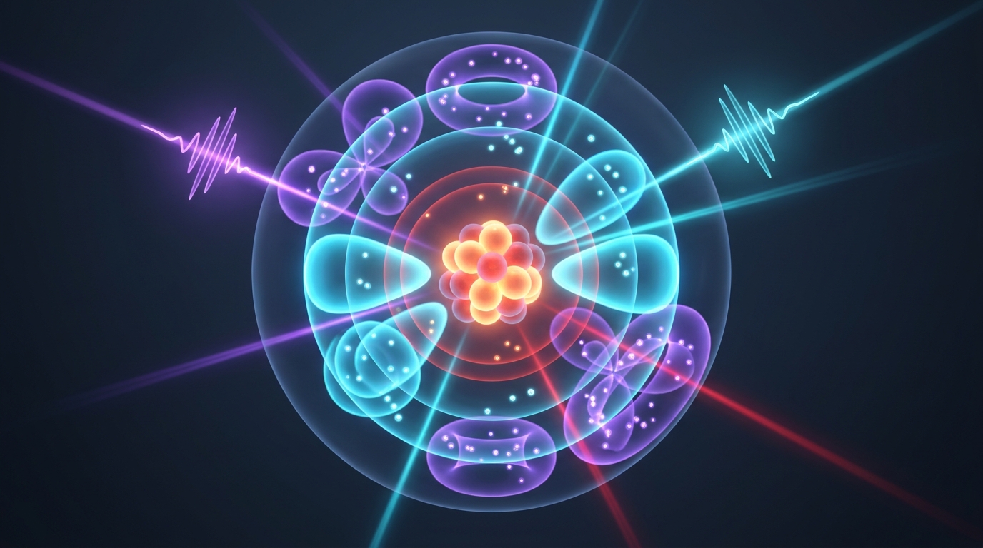
Ilustração tridimensional de pacotes de onda quânticos em azul-ciano e violeta incidindo sobre cascas esféricas concêntricas de confinamento e lóbulos de densidade de probabilidade em torno do núcleo

🌍 Ponto de Partida Químico e Ligação: Porque Precisamos Deste Capítulo?Chemical Starting Point & Connection: Why Do We Need This Chapter?

Se já fez uma cadeira de Química Geral ou de Química Orgânica, provavelmente aprendeu um conjunto de regras que parecem quase mágicas: o carbono faz quatro ligações tetraédricas a $109.5^\circ$, as orbitais chamam-se $1s, 2s, 2p, 3d$, cada orbital leva no máximo dois eletrões com spins opostos, o benzeno é extraordinariamente estável por ter $6$ eletrões $\pi$, e uma molécula absorve luz ultravioleta ou visível apenas em comprimentos de onda muito específicos. Mas já parou para perguntar: de onde vêm realmente estas regras? Porque é que um eletrão negativo não cai simplesmente para cima do núcleo positivo a que está atraído? If you have taken General or Organic Chemistry, you have learned a set of rules that can feel almost magical: carbon forms four tetrahedral bonds at $109.5^\circ$, orbitals are labeled $1s, 2s, 2p, 3d$, each orbital holds at most two opposite-spin electrons, benzene is unusually stable with $6$ $\pi$-electrons, and a molecule absorbs UV-Vis light only at specific wavelengths. Have you ever paused to ask: where do these rules actually come from? Why doesn't a negatively charged electron simply fall right into the positively charged nucleus attracting it?

Neste primeiro capítulo não vamos decorar fórmulas: vamos perceber porque é que a Física Clássica do nosso dia a dia falha completamente à escala de $1\text{ Å}$ e como a natureza ondulatória do eletrão explica a estabilidade de toda a matéria. Na segunda metade do capítulo, vamos aprender o «idioma universal» que todos os programas de Química Quântica (como o ORCA ou o Gaussian) utilizam nos seus ficheiros de output — as Unidades Atómicas de Hartree — para que saiba converter instantaneamente qualquer energia computacional para as unidades do seu laboratório ($\text{kcal/mol}$, $\text{kJ/mol}$ ou $\text{eV}$). In this opening chapter we will not memorize formulas blindly: we will understand why everyday Classical Physics breaks down completely at the $1\text{ Å}$ scale and how the wave nature of the electron explains the stability of all matter. In the second half of the chapter, we will learn the "universal language" spoken by every Quantum Chemistry package (such as ORCA or Gaussian) in its output files — Hartree Atomic Units — so you can effortlessly translate any computational energy into laboratory units ($\text{kcal/mol}$, $\text{kJ/mol}$, or $\text{eV}$).

1.1 O Mistério da Estabilidade Atómica: Porque é que os Átomos Não Colapsam em 16 Picossegundos? 1.1 The Mystery of Atomic Stability: Why Don't Atoms Collapse in 16 Picoseconds?

Em 1911, Ernest Rutherford descobriu que quase toda a massa do átomo está concentrada num núcleo positivo minúsculo, rodeado por eletrões negativos muito leves a uma distância de cerca de meio Ångström ($0.53\text{ Å}$). À primeira vista, é tentador imaginar o átomo de Hidrogénio como um «sistema solar em miniatura», onde o eletrão gira em redor do protão tal como a Terra gira em redor do Sol. Mas há uma diferença crucial entre a Terra e um eletrão: a Terra é eletricamente neutra, enquanto o eletrão transporta uma carga elétrica negativa! In 1911, Ernest Rutherford discovered that nearly all the mass of an atom is concentrated in a tiny positive nucleus, surrounded by light negative electrons about half an Ångström ($0.53\text{ Å}$) away. At first glance, it is tempting to picture the Hydrogen atom as a "miniature solar system", with the electron orbiting the proton just as the Earth orbits the Sun. Yet there is one crucial difference between the Earth and an electron: the Earth is electrically neutral, whereas the electron carries an electric charge!

Comparação tridimensional entre o colapso espiral eletrodinâmico clássico de Rutherford em 16 picossegundos (esquerda, em âmbar) e a estabilidade quântica por ondas estacionárias 3D em torno do núcleo (direita, em azul-ciano) — **Ilustração Científica 1.1 (Clique na imagem para ampliar):** O paradoxo da estabilidade atómica. **À esquerda (Física Clássica — Laranja/Âmbar):** um eletrão clássico em órbita curvilínea sofre aceleração centrípeta contínua, irradia energia eletromagnética (ondas de Larmor) e cai em espiral para o núcleo em apenas $\tau \approx 16\text{ ps}$. **À direita (Mecânica Quântica — Azul-Ciano):** o eletrão comporta-se como uma onda estacionária tridimensional ($\psi_{n\ell m}$) confinada em torno do núcleo a $a_0 = 0.53\text{ Å}$, cujo estado fundamental não irradia nem pode colapsar. **Scientific Illustration 1.1 (Click image to zoom):** The paradox of atomic stability. **Left (Classical Physics — Amber):** a classical orbiting electron undergoes continuous centripetal acceleration, radiates electromagnetic energy (Larmor waves), and spirals into the nucleus in just $\tau \approx 16\text{ ps}$. **Right (Quantum Mechanics — Cyan):** the electron exists as a 3D standing wave ($\psi_{n\ell m}$) confined around the nucleus at $a_0 = 0.53\text{ Å}$, whose ground state neither radiates nor collapses.

Segundo as leis do Eletromagnetismo Clássico de James Clerk Maxwell (que são exatamente o princípio físico pelo qual a antena do seu telemóvel ou de uma estação de rádio funciona!), qualquer carga elétrica acelerada é obrigada a emitir radiação eletromagnética (luz). Ora, um eletrão em movimento circular em redor do núcleo está sempre a mudar de direção, pelo que sofre uma aceleração centrípeta enorme ($a_c = v^2 / r \approx 9 \times 10^{22}\text{ m/s}^2$). Pela fórmula de Larmor da eletrodinâmica clássica, o eletrão perderia energia cinética a cada volta e descreveria uma espiral mortal para dentro do núcleo (como ilustrado no lado esquerdo da figura acima), destruindo o átomo de Hidrogénio num intervalo de tempo fácil de calcular: According to James Clerk Maxwell's laws of Classical Electromagnetism (the exact physical principle behind every radio and mobile-phone antenna!), any accelerated electric charge must emit electromagnetic radiation (light). An electron moving in a circle around a nucleus is constantly changing direction and therefore experiences a huge centripetal acceleration ($a_c = v^2 / r \approx 9 \times 10^{22}\text{ m/s}^2$). By the classical Larmor radiation formula, the electron would lose kinetic energy on every turn and trace a death spiral into the nucleus (as shown on the left side of the illustration above), destroying the Hydrogen atom in a time interval given by:

POTÊNCIA IRRADIADA DE LARMOR E TEMPO DE COLAPSO CLÁSSICO DO ÁTOMO DE HIDROGÉNIOLARMOR RADIATED POWER & CLASSICAL COLLAPSE TIME OF THE HYDROGEN ATOM $$P_{\text{Larmor}} = \frac{e^2\,a_c^2}{6\pi\varepsilon_0\,c^3} \qquad \Longrightarrow \qquad \tau_{\text{colapso}} = \frac{m_e^2\,r_0^3\,(4\pi\varepsilon_0)^2\,c^3}{4\,e^4} \approx 1.56 \times 10^{-11}\text{ s} \approx \mathbf{16\text{ picossegundos}}$$

Se a Física Clássica estivesse certa à escala atómica, todos os átomos do Universo — incluindo o ADN e as proteínas do seu corpo — colapsariam num clarão de radiação ultravioleta em 16 bilionésimos de segundo ($16\text{ ps}$), e os átomos emitiriam um espetro contínuo em vez das riscas discretas observadas experimentalmente! Foi para resolver esta catástrofe que Max Planck (1900, quantização da energia $\Delta E = h\nu$), Albert Einstein (1905, efeito fotoelétrico $K_{\max} = h\nu - \Phi$) e Niels Bohr (1913, órbitas estacionárias quantizadas $E_n = -13.6\text{ eV}/n^2$) abriram caminho à solução definitiva (lado direito da figura): o eletrão atómico não é um ponto clássico em órbita, mas sim uma onda estacionária tridimensional sustentada pelo princípio da incerteza! If Classical Physics held at the atomic scale, every atom in the Universe — including the DNA and proteins in your body — would collapse in a flash of ultraviolet radiation within 16 trillionths of a second ($16\text{ ps}$), emitting a continuous smear of frequencies rather than sharp spectral lines! Resolving this catastrophe led Max Planck (1900, energy quantization $\Delta E = h\nu$), Albert Einstein (1905, photoelectric effect $K_{\max} = h\nu - \Phi$), and Niels Bohr (1913, quantized stationary states $E_n = -13.6\text{ eV}/n^2$) to the quantum solution (right side of the figure): the atomic electron is not a classical orbiting point charge, but a three-dimensional standing wave stabilized by the uncertainty principle!

1.2 A Ideia Genial de Louis de Broglie (1924): Porque os Eletrões São Ondas e as Bolas de Ténis Não? 1.2 Louis de Broglie's Brilliant Idea (1924): Why Are Electrons Waves While Tennis Balls Are Not?

Se os eletrões nos átomos só podem ocupar degraus discretos de energia, que tipo de objeto físico se comporta naturalmente assim? Em 1924, o jovem físico francês Louis de Broglie fez uma ligação simples e revolucionária: no nosso mundo quotidiano, as ondas presas num espaço finito só conseguem vibrar em frequências discretas (pense numa corda de guitarra presa nas duas pontas, que só pode vibrar na nota fundamental, no primeiro harmónico, no segundo harmónico, etc., porque tem de ter um número inteiro de meias-ondas entre as extremidades!). If electrons inside atoms can occupy only discrete energy rungs, what kind of physical object naturally behaves that way? In 1924, the young French physicist Louis de Broglie made a simple, revolutionary connection: in our everyday world, waves confined to a finite space can vibrate only at discrete frequencies (think of a guitar string clamped at both ends, which can vibrate only in its fundamental tone, first overtone, second overtone, etc., because an integer number of half-wavelengths must fit between the clamps!).

Analogia de Louis de Broglie: das ondas estacionárias numa corda vibrante presa nas extremidades (esquerda: fundamental, primeiro e segundo harmónicos) à onda estacionária circular de matéria em torno do núcleo atómico (direita: onda construtiva fechada em azul-ciano versus onda destrutiva fora de fase em âmbar) — **Ilustração Científica 1.2 (Clique na imagem para ampliar):** Da corda vibrante à quantização atómica de Louis de Broglie. **À esquerda:** uma onda confinada entre dois apoios fixos só pode vibrar em modos discretos com um número inteiro de meias-ondas ($n = 1, 2, 3,\dots$, separados por nós onde a amplitude é nula). **À direita:** quando a onda de matéria do eletrão se fecha em torno do núcleo atómico, apenas os raios cujo perímetro acomoda um número inteiro de comprimentos de onda ($2\pi r = n\lambda_{\text{dB}}$, anel azul-ciano luminoso) interferem construtivamente e sobrevivem como estados estacionários; qualquer comprimento fracionário (onda exterior em âmbar/vermelho) fecha fora de fase e anula-se por interferência destrutiva. **Scientific Illustration 1.2 (Click image to zoom):** From a clamped vibrating string to Louis de Broglie's atomic quantization. **Left:** a wave confined between two fixed supports can vibrate only in discrete modes containing an integer number of half-wavelengths ($n = 1, 2, 3,\dots$, separated by nodes of zero amplitude). **Right:** when the electron's matter wave wraps around the atomic nucleus, only radii whose circumference accommodates an integer number of wavelengths ($2\pi r = n\lambda_{\text{dB}}$, bright cyan ring) interfere constructively and survive as stationary states; any fractional wavelength (outer amber/red wave) fails to close in phase and cancels by destructive interference.

De Broglie propôs então que o eletrão não é uma «bolinha dura» a rodar em torno do núcleo: toda a partícula de matéria com massa $m$ e velocidade $v$ (momento linear $p = mv$) tem um comprimento de onda intrínseco $\lambda_{\text{dB}}$, dado pelo quociente entre a constante de Planck $h$ e o seu momento linear $p$: De Broglie therefore proposed that the electron is not a tiny hard marble orbiting the nucleus: every particle of matter with mass $m$ and speed $v$ (linear momentum $p = mv$) has an intrinsic wavelength $\lambda_{\text{dB}}$, given by Planck's constant $h$ divided by its momentum $p$:

COMPRIMENTO DE ONDA DE DE BROGLIE E CONDIÇÃO DE ONDA ESTACIONÁRIA ATÓMICADE BROGLIE WAVELENGTH & ATOMIC STANDING-WAVE CONDITION $$\lambda_{\text{dB}} = \frac{h}{p} = \frac{h}{m v} = \frac{h}{\sqrt{2 m K}} \qquad \Longrightarrow \qquad 2\pi r = n\,\lambda_{\text{dB}} \;\;\;(n = 1, 2, 3, \dots)$$

🗣️ O que esta equação significa sem matemática:What this equation means without math:
Repare onde está a massa $m$: está no denominador! Isto significa que quanto mais leve for uma partícula, maior é o seu comprimento de onda $\lambda_{\text{dB}}$ e mais «espalhada» e ondulatória ela é. Sempre que o comprimento de onda $\lambda_{\text{dB}}$ de uma partícula for da mesma ordem de grandeza (ou maior) do que a «caixa» ou molécula onde ela se move, a partícula deixa de se comportar como uma bolinha clássica e passa a comportar-se como uma onda estacionária tridimensional (uma orbital!). Notice where the mass $m$ sits: in the denominator! This means that the lighter a particle is, the longer its wavelength $\lambda_{\text{dB}}$ and the more spread-out and wave-like it becomes. Whenever a particle's wavelength $\lambda_{\text{dB}}$ is comparable to (or larger than) the "box" or molecule confining it, the particle stops behaving like a classical marble and acts as a three-dimensional standing wave (an orbital!).

1. Eletrão num Átomo ($m_e = 9.11\times 10^{-31}\text{ kg}$)1. Electron in an Atom ($m_e = 9.11\times 10^{-31}\text{ kg}$)

Com velocidade típica $v \approx 2.19 \times 10^6\text{ m/s}$ no átomo de H, obtemos $\lambda_{\text{dB}} = \mathbf{3.32\text{ Å}}$! Como $\lambda_{\text{dB}} = 3.32\text{ Å}$ é maior do que o próprio átomo ($\sim 1\text{ Å}$), o eletrão é 100% quântico e ondulatório! With typical speed $v \approx 2.19 \times 10^6\text{ m/s}$ in the H atom, we obtain $\lambda_{\text{dB}} = \mathbf{3.32\text{ Å}}$! Because $\lambda_{\text{dB}} = 3.32\text{ Å}$ is larger than the atom itself ($\sim 1\text{ Å}$), the electron is 100% quantum and wave-like!

2. Protão Térmico ($^1\text{H}^+$, $m_p = 1836\,m_e$)2. Thermal Proton ($^1\text{H}^+$, $m_p = 1836\,m_e$)

Apesar de ser $1836$ vezes mais pesado do que o eletrão, à temperatura ambiente ($298\text{ K}$) um protão ou átomo de H tem $\lambda_{\text{dB}} \approx \mathbf{1.46\text{ Å}}$. Por isso, transferências de protão e hidreto em enzimas também têm efeitos quânticos (energia de ponto zero e efeito de túnel)! Although $1836$ times heavier than an electron, at room temperature ($298\text{ K}$) a proton or H atom still has $\lambda_{\text{dB}} \approx \mathbf{1.46\text{ Å}}$. Consequently, proton and hydride transfers in enzymes also show quantum effects (zero-point energy and tunnelling)!

3. Bola de Ténis ($m = 0.06\text{ kg}$, $v = 20\text{ m/s}$)3. Tennis Ball ($m = 0.06\text{ kg}$, $v = 20\text{ m/s}$)

Para objetos macroscópicos, a massa no denominador é gigantesca e dá $\lambda_{\text{dB}} \approx \mathbf{5.5 \times 10^{-34}\text{ m}}$ ($10^{24}$ vezes mais pequeno do que um átomo!). É por isso que nunca vemos uma bola de ténis difratar ou fazer efeito de túnel através da rede! For macroscopic objects, the huge mass in the denominator gives $\lambda_{\text{dB}} \approx \mathbf{5.5 \times 10^{-34}\text{ m}}$ ($10^{24}$ times smaller than an atom!). That is why we never see a tennis ball diffract or tunnel through the net!

1.3 Unidades Atómicas de Hartree ($m_e = e = \hbar = 4\pi\varepsilon_0 = 1$): A «Moeda Natural do Átomo» 1.3 Hartree Atomic Units ($m_e = e = \hbar = 4\pi\varepsilon_0 = 1$): The "Natural Currency of the Atom"

Imagine que ia comprar um café ou medir a massa de um comprimido farmacêutico, mas era obrigado a exprimir todos os pesos em «massas solares» ($1.99 \times 10^{30}\text{ kg}$) e todos os comprimentos em «anos-luz» ($9.46 \times 10^{15}\text{ m}$): teria de arrastar potências de $10^{-33}$ em cada conta! Ora, para um eletrão dentro de uma molécula, usar as unidades humanas do Sistema Internacional (quilogramas, metros, segundos e Coulombs) é igualmente absurdo, porque um eletrão pesa $9.109 \times 10^{-31}\text{ kg}$, tem carga $1.602 \times 10^{-19}\text{ C}$ e a constante de Planck reduzida vale $\hbar = 1.055 \times 10^{-34}\text{ J}\cdot\text{s}$. Imagine buying a cup of coffee or weighing a pharmaceutical tablet while being forced to express every weight in "solar masses" ($1.99 \times 10^{30}\text{ kg}$) and every length in "light-years" ($9.46 \times 10^{15}\text{ m}$): you would have to drag powers of $10^{-33}$ through every single calculation! For an electron inside a molecule, using everyday human SI units (kilograms, meters, seconds, and Coulombs) is just as awkward, because an electron weighs $9.109 \times 10^{-31}\text{ kg}$, carries charge $1.602 \times 10^{-19}\text{ C}$, and has reduced Planck constant $\hbar = 1.055 \times 10^{-34}\text{ J}\cdot\text{s}$.

💬 Dúvida Frequente · Porque é que os programas usam Hartree e bohr em vez de kJ/mol e Ångström?💬 Student Q&A · Why do programs use Hartree and bohr instead of kJ/mol and Ångström?

Em unidades atómicas, as constantes fundamentais que aparecem em todas as equações ($\hbar$, a massa do eletrão, a carga elementar e $4\pi\varepsilon_0$) valem exatamente 1. As equações ficam muito mais curtas e os números típicos ficam perto de 1, o que reduz erros. A energia do átomo de Hidrogénio, por exemplo, é simplesmente $-0{,}5\text{ E}_\text{h}$. Só tem de converter no fim: $1\text{ E}_\text{h} = 627{,}5\text{ kcal/mol} = 2625{,}5\text{ kJ/mol} = 27{,}211\text{ eV}$ e $1\ a_0 = 0{,}529\text{ Å}$. Guarde estas quatro conversões: vai usá-las em todos os outputs do ORCA.In atomic units, the fundamental constants that appear in every equation ($\hbar$, the electron mass, the elementary charge, and $4\pi\varepsilon_0$) are exactly 1. Equations become much shorter and typical numbers are close to 1, which reduces mistakes. The energy of the Hydrogen atom, for example, is simply $-0.5\text{ E}_\text{h}$. You only convert at the end: $1\text{ E}_\text{h} = 627.5\text{ kcal/mol} = 2625.5\text{ kJ/mol} = 27.211\text{ eV}$ and $1\ a_0 = 0.529\text{ Å}$. Keep these four conversions handy: you will use them on every ORCA output.

Em 1928, o físico britânico Douglas Hartree teve uma ideia prática brilhante: em vez de usarmos o metro e o quilograma nas equações da Química Quântica, porque não usamos o próprio átomo de Hidrogénio como régua e balança? Se definirmos a massa de $1$ eletrão como a nossa unidade de massa ($m_e = 1$), a carga elementar como a unidade de carga ($e = 1$), o quantum de momento angular como $\hbar = 1$ e a constante eletrostática como $\frac{1}{4\pi\varepsilon_0} = 1$, todas essas constantes desaparecem das equações! In 1928, the British physicist Douglas Hartree had a brilliant practical idea: instead of using the meter and the kilogram in Quantum Chemistry equations, why not use the Hydrogen atom itself as our ruler and scale? By defining the mass of $1$ electron as our unit of mass ($m_e = 1$), the elementary charge as our unit of charge ($e = 1$), the angular momentum quantum as $\hbar = 1$, and the electrostatic constant as $\frac{1}{4\pi\varepsilon_0} = 1$, all four clumsy constants vanish from the equations!

💡 Analogia: Contar Ovos às Dúzias ou Moléculas em MolesAnalogy: Counting Eggs by the Dozen or Molecules in Moles
Mudar do Sistema Internacional (SI) para Unidades Atómicas (a.u.) é exatamente como deixar de contar moléculas uma a uma ($6.022 \times 10^{23}$) e passar a contar em moles ($\text{mol}$)! Nas unidades atómicas de Hartree:
• A unidade natural de distância chama-se $1\text{ Bohr}$ ($1\,a_0 = 0.529177\text{ Å}$), que é exatamente o raio mais provável da orbital $\text{1s}$ do átomo de Hidrogénio;
• A unidade natural de energia chama-se $1\text{ Hartree}$ ($1\text{ E}_\text{h} = 627.5095\text{ kcal/mol} = 2625.50\text{ kJ/mol} = 27.2114\text{ eV}$), que é a repulsão eletrostática entre dois eletrões separados por $1\text{ Bohr}$ (e o dobro da energia de ionização do átomo de Hidrogénio, cuja energia exata no estado fundamental é $E_{\text{H}} = -\frac{1}{2}\text{ E}_\text{h} = -0.500000\text{ E}_\text{h}$!). Switching from SI units to Atomic Units (a.u.) is just like counting molecules in moles ($\text{mol}$) instead of individual particles ($6.022 \times 10^{23}$)! In Hartree atomic units:
• The natural unit of distance is $1\text{ Bohr}$ ($1\,a_0 = 0.529177\text{ Å}$), which is the exact most probable radius of the Hydrogen $\text{1s}$ orbital;
• The natural unit of energy is $1\text{ Hartree}$ ($1\text{ E}_\text{h} = 627.5095\text{ kcal/mol} = 2625.50\text{ kJ/mol} = 27.2114\text{ eV}$), which is the electrostatic repulsion between two electrons separated by $1\text{ Bohr}$ (and twice the ionization energy of the Hydrogen atom, whose exact ground-state energy is $E_{\text{H}} = -\frac{1}{2}\text{ E}_\text{h} = -0.500000\text{ E}_\text{h}$!).

📐 Veja Como a Equação de Schrödinger Fica Limpa em Unidades Atómicas See How Clean the Schrödinger Equation Becomes in Atomic Units

Em unidades SI, a equação da energia de um eletrão atraído por um núcleo de número atómico $Z$ está cheia de constantes ($\hbar^2, m_e, e^2, 4\pi\varepsilon_0$). Mas quando medimos comprimentos em Bohrs ($a_0 = \frac{4\pi\varepsilon_0\hbar^2}{m_e e^2} = 0.529177\text{ Å}$) e energias em Hartrees ($E_{\text{h}} = \frac{\hbar^2}{m_e a_0^2} = 27.2114\text{ eV}$), a mesma equação simplifica imediatamente para: In SI units, the energy equation for an electron attracted by a nucleus of atomic number $Z$ is crowded with constants ($\hbar^2, m_e, e^2, 4\pi\varepsilon_0$). When we measure lengths in Bohrs ($a_0 = \frac{4\pi\varepsilon_0\hbar^2}{m_e e^2} = 0.529177\text{ Å}$) and energies in Hartrees ($E_{\text{h}} = \frac{\hbar^2}{m_e a_0^2} = 27.2114\text{ eV}$), the exact same equation simplifies immediately to:

$$\underbrace{\left( -\frac{\hbar^2}{2 m_e}\nabla^2 - \frac{Z e^2}{4\pi\varepsilon_0 r} \right)\psi = E\,\psi}_{\text{Em Unidades SI (Carregada de Constantes)}} \quad\xrightarrow{m_e = e = \hbar = 4\pi\varepsilon_0 = 1}\quad \underbrace{\left( -\frac{1}{2}\nabla^2 - \frac{Z}{r} \right)\psi = E\,\psi}_{\text{Em Unidades Atómicas de Hartree (Universal!)}}$$ $$\underbrace{\left( -\frac{\hbar^2}{2 m_e}\nabla^2 - \frac{Z e^2}{4\pi\varepsilon_0 r} \right)\psi = E\,\psi}_{\text{In SI Units (Crowded with Constants)}} \quad\xrightarrow{m_e = e = \hbar = 4\pi\varepsilon_0 = 1}\quad \underbrace{\left( -\frac{1}{2}\nabla^2 - \frac{Z}{r} \right)\psi = E\,\psi}_{\text{In Hartree Atomic Units (Universal!)}}$$

💬 Dúvida de Estudante: «Porque é que as energias eletrónicas nos outputs do ORCA e do Gaussian são sempre números negativos grandes (por exemplo, $-0.500\text{ E}_\text{h}$ para o átomo de H ou $-76.4\text{ E}_\text{h}$ para a molécula de água)?»Student Question: "Why are electronic energies in ORCA and Gaussian output files always large negative numbers (for instance, $-0.500\text{ E}_\text{h}$ for the H atom or $-76.4\text{ E}_\text{h}$ for a water molecule)?" Excelente pergunta! Em Química Quântica, o zero de energia ($E = 0$) é definido por convenção como o estado em que todos os núcleos e todos os eletrões estão infinitamente afastados uns dos outros e em repouso. Quando os eletrões negativos se aproximam dos núcleos positivos para formar átomos e moléculas, o sistema liberta uma enorme quantidade de energia eletrostática e desce para um «poço de potencial» estável. Por isso, qualquer átomo ou molécula ligada tem obrigatoriamente energia total negativa ($E \lt 0$), e quanto mais negativa for a energia, mais estável é o sistema! Great question! In Quantum Chemistry, the zero of energy ($E = 0$) is defined by convention as the state where all nuclei and all electrons are infinitely separated from one another and at rest. When negative electrons come together around positive nuclei to form atoms and molecules, the system releases a huge amount of electrostatic energy and drops into a stable potential well. Thus, any bound atom or molecule necessarily has a negative total energy ($E \lt 0$), and the more negative the energy, the more stable the system!

1.4 Tabela de Conversão para o Laboratório, «Precisão Química» ($1\text{ kcal/mol}$) e Simulador Interativo 1.1 1.4 Laboratory Conversion Table, "Chemical Accuracy" ($1\text{ kcal/mol}$) & Interactive Simulator 1.1

Como $1\text{ Hartree}$ ($627.51\text{ kcal/mol}$) é uma unidade de energia enorme — maior do que a energia de quase qualquer ligação covalente simples! —, uma pequena diferença no 3.º ou 4.º algarismo decimal de um cálculo em Hartrees tem um impacto dramático na velocidade de uma reação química ou na ligação de um fármaco a uma proteína. Because $1\text{ Hartree}$ ($627.51\text{ kcal/mol}$) is a huge unit of energy — larger than the bond energy of almost any single covalent bond! — a tiny change in the 3rd or 4th decimal place of a Hartree energy has a dramatic impact on a chemical reaction rate or drug-protein binding affinity.

Em Termodinâmica e Cinética Química à temperatura ambiente ($T = 298.15\text{ K}$, onde a energia térmica $RT$ vale cerca de $0.592\text{ kcal/mol} = 2.479\text{ kJ/mol}$), a constante de equilíbrio $K_{\text{eq}} = e^{-\Delta G^\circ / RT}$ e a constante de velocidade $k(T) \propto e^{-\Delta G^\ddagger / RT}$ dependem exponencialmente da energia. Basta um erro de $\mathbf{1.36\text{ kcal/mol}}$ ($5.71\text{ kJ/mol}$) para errar a velocidade de uma reação ou o $K_d$ de um fármaco num fator de $10$ vezes! Por isso, a comunidade científica define $1.0\text{ kcal/mol} \approx 0.001594\text{ E}_\text{h} \approx 1.6\text{ mE}_\text{h}$ como a fasquia de ouro chamada «Precisão Química» (Chemical Accuracy). In Chemical Thermodynamics and Kinetics at room temperature ($T = 298.15\text{ K}$, where thermal energy $RT$ is $0.592\text{ kcal/mol} = 2.479\text{ kJ/mol}$), the equilibrium constant $K_{\text{eq}} = e^{-\Delta G^\circ / RT}$ and rate constant $k(T) \propto e^{-\Delta G^\ddagger / RT}$ depend exponentially on energy. An error of just $\mathbf{1.36\text{ kcal/mol}}$ ($5.71\text{ kJ/mol}$) shifts a reaction rate or a drug's binding constant $K_d$ by a factor of $10\times$! Consequently, the scientific community defines $1.0\text{ kcal/mol} \approx 0.001594\text{ E}_\text{h} \approx 1.6\text{ mE}_\text{h}$ as the gold-standard benchmark known as "Chemical Accuracy".

Grandeza FísicaPhysical Quantity	Unidade Atómica (Símbolo)Atomic Unit (Symbol)	Equivalência em Unidades de Laboratório e SIEquivalence in Laboratory & SI Units	Significado Químico IntuitivoIntuitive Chemical Meaning
ComprimentoLength	$1\,a_0$ (1 Bohr)	$\mathbf{0.529177\text{ Å}} = 52.918\text{ pm}$	Raio mais provável da orbital $\text{1s}$ do átomo de $\text{H}$. Uma ligação $\text{C–C}$ ($1.54\text{ Å}$) mede $\approx 2.91\,a_0$.Most probable radius of the $\text{H}$ $\text{1s}$ orbital. A $\text{C–C}$ bond ($1.54\text{ Å}$) is $\approx 2.91\,a_0$.
EnergiaEnergy	$1\text{ E}_\text{h}$ (1 Hartree)	$\mathbf{627.5095\text{ kcal/mol}} = \mathbf{2625.50\text{ kJ/mol}} = \mathbf{27.2114\text{ eV}}$	Dobro da energia de ionização do átomo de $\text{H}$ ($E_{1s} = -0.5000\text{ E}_\text{h} = -313.75\text{ kcal/mol}$).Twice the ionization energy of the $\text{H}$ atom ($E_{1s} = -0.5000\text{ E}_\text{h} = -313.75\text{ kcal/mol}$).
«Precisão Química»"Chemical Accuracy"	$\mathbf{1.5936\text{ mE}_\text{h}} = 0.001594\text{ E}_\text{h}$	$\mathbf{1.00\text{ kcal/mol}} = 4.184\text{ kJ/mol} = 0.0434\text{ eV}$	Meta de exatidão termoquímica: erro máximo aceitável para prever barreiras e equilíbrios à temperatura ambiente.Thermochemical target: maximum acceptable error for predicting room-temperature barriers and equilibria.
TempoTime	$\tau_0 = \hbar/E_{\text{h}} = 1\text{ u.a.}$	$\mathbf{24.189\text{ as}} = 0.0242\text{ fs}$	Escala temporal natural do movimento dos eletrões (attosegundos), mil vezes mais rápida que as vibrações nucleares (femtossegundos).Natural timescale of electron motion (attoseconds), a thousand times faster than nuclear vibrations (femtoseconds).

🔬 Interativo 1.1🔬 Interactive 1.1 Calculadora de Comprimento de Onda de de Broglie, Unidades Atómicas e Escala Quântica de Broglie Wavelength, Atomic Units & Quantum Scale Calculator

🎯 O Que Se Pretende Fazer Neste Simulador e Porquê What This Simulator Does & Why It Matters

Objetivo: Comprovar na prática a hipótese de Louis de Broglie ($\lambda_{\text{dB}} = h/p$) e as Unidades Atómicas de Hartree. O que pretende fazer: Comparar o comprimento de onda $\lambda_{\text{dB}}$ (a onda azul no gráfico) com o diâmetro do átomo de Hidrogénio ($1.06\text{ Å}$) e de uma ligação $\text{C–C}$ ($1.54\text{ Å}$). Sempre que $\lambda_{\text{dB}}$ é maior ou comparável ao átomo, a física clássica colapsa e a partícula comporta-se como uma orbital quântica! Experimente os botões rápidos abaixo ou clique em cada seletor para ver a explicação. Goal: Test Louis de Broglie's hypothesis ($\lambda_{\text{dB}} = h/p$) and Hartree Atomic Units hands-on. What to do: Compare the de Broglie wavelength $\lambda_{\text{dB}}$ (blue wave in the plot) against the diameter of a Hydrogen atom ($1.06\text{ Å}$) and a $\text{C–C}$ bond ($1.54\text{ Å}$). Whenever $\lambda_{\text{dB}}$ is comparable to or larger than the atom, classical physics fails and the particle behaves as a quantum orbital! Try the quick preset buttons below or click each selector's explanation.

Partícula / Objeto:Particle / Object:

ℹ️ Explicação deste seletor / controlo (clique para abrir)ℹ️ Explanation of this selector / control (click to open)

O que faz este seletor: Escolhe a partícula cuja onda de matéria $\lambda_{\text{dB}} = h/p = h/\sqrt{2mK}$ queremos calcular e comparar com o tamanho de um átomo ($1.06\text{ Å}$) e de uma ligação $\text{C–C}$ ($1.54\text{ Å}$).
O que observar: Mude de Eletrão para Protão, Deuterão e Carbono-12: verá que ao aumentar a massa $m$ no denominador, o comprimento de onda $\lambda_{\text{dB}}$ encolhe drasticamente (por um fator $\sqrt{m}$), explicando porque é que os eletrões são ondas deslocalizadas enquanto os átomos pesados de carbono se comportam quase como esferas localizadas!What this selector does: Selects the particle whose de Broglie matter wavelength $\lambda_{\text{dB}} = h/p = h/\sqrt{2mK}$ is calculated and compared against the diameter of an H atom ($1.06\text{ Å}$) and a $\text{C–C}$ bond ($1.54\text{ Å}$).
What to observe: Switch from Electron to Proton, Deuteron, and Carbon-12: increasing mass $m$ in the denominator shrinks $\lambda_{\text{dB}}$ by $1/\sqrt{m}$, explaining why electrons are delocalized waves whereas heavy carbon nuclei behave nearly classically!

Energia Cinética $K$ (em $\text{eV}$):Kinetic Energy $K$ (in $\text{eV}$): 13.60 eV

ℹ️ Explicação deste seletor / controlo (clique para abrir)ℹ️ Explanation of this selector / control (click to open)

O que controla: Define a energia cinética $K$ da partícula em eletrão-Volts ($\text{eV}$). Por defeito está em $13.60\text{ eV}$ (a energia cinética média do eletrão $1s$ no átomo de Hidrogénio).
O que observar: Aumentar $K$ aumenta a velocidade $v$ e o momento linear $p = \sqrt{2mK}$, tornando a onda azul no gráfico mais curta e comprimida (menor $\lambda_{\text{dB}}$); diminuir $K$ (ex.: energias térmicas $\sim 0.04\text{ eV}$) alarga $\lambda_{\text{dB}}$ até que até o protão $^1\text{H}^+$ fica com $\lambda_{\text{dB}} > 1\text{ Å}$!What it controls: Sets the particle's kinetic energy $K$ in electron-volts ($\text{eV}$). Defaults to $13.60\text{ eV}$ (the mean kinetic energy of the $1s$ electron in the Hydrogen atom).
What to observe: Raising $K$ increases speed $v$ and momentum $p = \sqrt{2mK}$, compressing the blue wave in the plot (shorter $\lambda_{\text{dB}}$); lowering $K$ toward thermal energies ($\sim 0.04\text{ eV}$) stretches $\lambda_{\text{dB}}$ so that even a proton $^1\text{H}^+$ exceeds $1\text{ Å}$!

Diferença de Energia $\Delta E$ ($\text{kcal/mol}$):Energy Difference $\Delta E$ ($\text{kcal/mol}$): 12.0 kcal/mol

ℹ️ Explicação deste seletor / controlo (clique para abrir)ℹ️ Explanation of this selector / control (click to open)

O que controla: Define uma diferença de energia química $\Delta E$ em $\text{kcal/mol}$ (por exemplo, uma barreira de reação ou energia de ligação) para converter imediatamente para Unidades Atómicas de Hartree ($\text{E}_\text{h}$), $\text{kJ/mol}$ e $\text{eV}$.
O que observar: Ajuste para $1.0\text{ kcal/mol}$ para ver a fasquia de «Precisão Química» ($0.001594\text{ E}_\text{h} = 1.594\text{ mE}_\text{h}$) nos outputs do ORCA e Gaussian.What it controls: Sets a chemical energy difference $\Delta E$ in $\text{kcal/mol}$ (such as a reaction barrier or binding energy) for instant conversion into Hartree atomic units ($\text{E}_\text{h}$), $\text{kJ/mol}$, and $\text{eV}$.
What to observe: Set to $1.0\text{ kcal/mol}$ to inspect the "Chemical Accuracy" benchmark ($0.001594\text{ E}_\text{h} = 1.594\text{ mE}_\text{h}$) in ORCA and Gaussian outputs.

$\lambda_{\text{dB}} = h/\sqrt{2mK}$

3.325 Å (6.28 a₀)

Velocidade $v$Speed $v$

2.19×10⁶ m/s (1.00 a.u.)

$\Delta E$ em Hartree ($\text{E}_\text{h}$)$\Delta E$ in Hartree ($\text{E}_\text{h}$)

0.019123 Eh

$\Delta E$ em $\text{kJ/mol}$ & $\text{eV}$$\Delta E$ in $\text{kJ/mol}$ & $\text{eV}$

50.21 kJ/mol | 0.520 eV

⚡ Experiências Rápidas (Clique para Testar):⚡ Quick Experiments (Click to Test):

📌 Mensagens-Chave para o Químico (Resumo sem Matemática) — Capítulo 1Key Takeaways for Chemists (Math-Free Summary) — Chapter 1

Os eletrões nas moléculas não são bolinhas em órbita: Pela relação de de Broglie ($\lambda = h/p$), a massa pequeníssima do eletrão dá-lhe um comprimento de onda ($\sim 3.3\text{ Å}$) maior do que o próprio átomo, obrigando-o a comportar-se como uma onda estacionária 3D (uma orbital).Electrons in molecules are not orbiting marbles: By de Broglie's relation ($\lambda = h/p$), the electron's tiny mass gives it a wavelength ($\sim 3.3\text{ Å}$) larger than the atom itself, forcing it to behave as a 3D standing wave (an orbital).
Protões e átomos de Hidrogénio também são quânticos: Mesmo sendo $1836\times$ mais pesado do que um eletrão, o núcleo de $^1\text{H}$ ainda tem um comprimento de onda de $\sim 1.5\text{ Å}$ a $298\text{ K}$, razão pela qual as ligações $\text{C–H}$ e $\text{O–H}$ exibem forte Energia de Ponto Zero e efeito de túnel em enzimas.Protons and Hydrogen atoms are quantum too: Even though $1836\times$ heavier than an electron, the $^1\text{H}$ nucleus still has a wavelength of $\sim 1.5\text{ Å}$ at $298\text{ K}$, which is why $\text{C–H}$ and $\text{O–H}$ bonds exhibit strong Zero-Point Energy and enzymatic tunnelling.
Unidades Atómicas limpam a matemática: Nos programas de Química Computacional, medimos distâncias em Bohrs ($1\,a_0 = 0.529\text{ Å}$) e energias em Hartrees ($1\text{ E}_\text{h} = 627.51\text{ kcal/mol} = 2625.5\text{ kJ/mol} = 27.21\text{ eV}$). A «Precisão Química» de $1\text{ kcal/mol}$ corresponde a $1.594\text{ mE}_\text{h}$.Atomic Units clean up the math: In Computational Chemistry software, we measure distances in Bohrs ($1\,a_0 = 0.529\text{ Å}$) and energies in Hartrees ($1\text{ E}_\text{h} = 627.51\text{ kcal/mol} = 2625.5\text{ kJ/mol} = 27.21\text{ eV}$). "Chemical Accuracy" ($1\text{ kcal/mol}$) equals $1.594\text{ mE}_\text{h}$.

🎯 Questionário de Conceitos Fundamentais — Capítulo 1 — Porque a Mecânica Quântica é Necessária em Química e as Unidades Atómicas de HartreeCore Concepts Questionnaire — Chapter 1 — Why Quantum Mechanics Is Needed in Chemistry & Hartree Atomic Units

Questões acessíveis sobre os conceitos essenciais deste capítulo • Clique em «Outra Variante» ou «Feedback de Estudo» para saber o que estudar mais.Accessible questions on this chapter's essential concepts • Click "Swap Variant" or "Study Feedback" for personalized study guidance.

0 / 4 (0%)

🔗 Texto de Ligação para o Capítulo 2Bridge to Chapter 2

Agora que já sabemos que os eletrões nas moléculas são ondas estacionárias tridimensionais e que medimos o mundo atómico em Bohrs e Hartrees, surge a pergunta prática: como é que descrevemos matematicamente essas ondas e como é que um computador calcula a sua energia e a sua forma? No Capítulo 2 vamos desmistificar passo a passo, sem qualquer receio, os quatro ingredientes da linguagem quântica — números complexos, a notação $\langle \phi | \psi \rangle$ de Dirac, os operadores Hermitianos e as matrizes que o computador diagonaliza. Now that we know electrons in molecules are three-dimensional standing waves and that we measure the atomic world in Bohrs and Hartrees, the practical question arises: how do we mathematically describe these waves, and how does a computer calculate their energy and shape? In Chapter 2 we will demystify step by step, without any fear, the four ingredients of quantum language — complex numbers, Dirac's $\langle \phi | \psi \rangle$ notation, Hermitian operators, and the matrices that computers diagonalize.

02

Capítulo 2 — Ferramentas Matemáticas para a Química Quântica (Sem Medo!) Chapter 2 — Mathematical Tools for Quantum Chemistry (Fear-Free!)

Um guia amigável e intuitivo para ler símbolos quânticos como quem lê português ou inglês: números complexos, espaços de Hilbert, bra-kets de Dirac, operadores Hermitianos e como uma equação diferencial se transforma numa tabela de números (matriz) no computador. A friendly, intuitive guide to reading quantum symbols like plain English or Portuguese: complex numbers, Hilbert spaces, Dirac bra-kets, Hermitian operators, and how a differential equation becomes a table of numbers (a matrix) on a computer.

🌍 Ponto de Partida Químico e Ligação: Porque Precisamos Deste Capítulo?Chemical Starting Point & Connection: Why Do We Need This Chapter?

A maior barreira que afasta muitos estudantes brilhantes de Química e Bioquímica da Mecânica Quântica não é a Física — é o susto visual ao abrir uma página e encontrar símbolos como $\Psi^*(\mathbf{r})$, $\langle \phi_m | \hat{H} | \phi_n \rangle$, $\nabla^2$ ou $\mathbf{H}\mathbf{C} = \mathbf{S}\mathbf{C}\boldsymbol{\varepsilon}$. Ninguém lhe explica que estes símbolos não foram inventados para complicar, mas sim como abreviaturas visuais muito simples! The biggest barrier keeping many bright Chemistry and Biochemistry students away from Quantum Mechanics is not the Physics — it is the visual shock of opening a page and seeing symbols like $\Psi^*(\mathbf{r})$, $\langle \phi_m | \hat{H} | \phi_n \rangle$, $\nabla^2$, or $\mathbf{H}\mathbf{C} = \mathbf{S}\mathbf{C}\boldsymbol{\varepsilon}$. Rarely does anyone explain that these symbols were not invented to make life harder, but rather as remarkably simple visual shorthands!

Neste capítulo vamos construir um «dicionário de tradução instantânea» entre a Química e a Matemática: vai ver que uma função de onda num espaço de Hilbert é exatamente como misturar cores primárias RGB ou combinar orbitais atómicas $s$ e $p$ para formar híbridos $sp^3$, que um operador $\hat{A}$ é apenas uma receita de cozinha aplicada a uma função, e que o trabalho de um supercomputador resume-se a diagonalizar uma tabela quadrada de números (uma matriz)! In this chapter we will build an "instant translation dictionary" between Chemistry and Mathematics: you will see that a wavefunction in Hilbert space is just like mixing RGB primary colors or combining $s$ and $p$ atomic orbitals into $sp^3$ hybrids, that an operator $\hat{A}$ is simply a recipe applied to a function, and that a supercomputer's job boils down to diagonalizing a square table of numbers (a matrix)!

2.1 Números Complexos ($z = x + iy = re^{i\theta}$) e Porque a Densidade $|\Psi|^2 = \Psi^\Psi$ É Sempre Real e Positiva 2.1 Complex Numbers ($z = x + iy = re^{i\theta}$) & Why the Density $|\Psi|^2 = \Psi^\Psi$ Is Always Real and Positive

Comecemos pela pergunta mais honesta de todas: se qualquer medição num laboratório de Química (uma energia de reação, um comprimento de ligação $\text{C=O}$, uma densidade eletrónica obtida por difração de raios X) dá sempre um número real, porque é que a função de onda $\Psi(\mathbf{r}, t)$ contém a unidade imaginária $i = \sqrt{-1}$ (onde $i^2 = -1$)? Let us start with the most honest question of all: if every measurement in a Chemistry lab (a reaction energy, a $\text{C=O}$ bond length, an electron density from X-ray diffraction) always yields a real number, why does the wavefunction $\Psi(\mathbf{r}, t)$ contain the imaginary unit $i = \sqrt{-1}$ (where $i^2 = -1$)?

A razão é que uma onda em movimento precisa de dois números em cada ponto do espaço: o seu tamanho (amplitude $r$) e o ângulo em que se encontra no seu ciclo de oscilação (fase $\theta$, que nos diz se duas ondas que se encontram vão somar-se construtivamente para criar uma ligação química ou cancelar-se destrutivamente num plano nodal!). A famosa fórmula de Euler ($e^{i\theta} = \cos\theta + i\sin\theta$) guarda a amplitude $r$ e a fase $\theta$ num único número complexo compacto $z = r e^{i\theta}$. The reason is that a wave in motion requires two pieces of information at every point in space: its height (amplitude $r$) and the angle of its oscillation cycle (phase $\theta$, which tells us whether two meeting waves will interfere constructively to form a chemical bond or cancel destructively at a nodal plane!). Leonhard Euler's famous formula ($e^{i\theta} = \cos\theta + i\sin\theta$) packs both amplitude $r$ and phase $\theta$ into a single compact complex number $z = r e^{i\theta}$.

💡 Analogia do Relógio: O Ponteiro que Roda no Plano ComplexoClock Analogy: The Rotating Hand in the Complex Plane
Imagine o ponteiro de um relógio de comprimento $r$: a sombra horizontal do ponteiro é a parte real $x = r\cos\theta$ e a sombra vertical é a parte imaginária $y = r\sin\theta$. Quando o tempo passa, o ponteiro roda suavemente ($e^{-i\omega t}$), mudando de direção ($\theta$), mas o comprimento do ponteiro $r$ mantém-se constante! Para descobrir o quadrado do comprimento real $r^2 = x^2 + y^2$ sem depender do ângulo $\theta$, basta multiplicar o número complexo $z = x + iy$ pelo seu conjugado complexo $z^* = x - iy$ (onde trocamos todos os $+i$ por $-i$): Picture a clock hand of length $r$: its horizontal shadow is the real part $x = r\cos\theta$ and its vertical shadow is the imaginary part $y = r\sin\theta$. As time passes, the clock hand rotates smoothly ($e^{-i\omega t}$), changing its angle ($\theta$), yet the length of the hand $r$ stays constant! To extract the real squared length $r^2 = x^2 + y^2$ independent of the angle $\theta$, we simply multiply the complex number $z = x + iy$ by its complex conjugate $z^* = x - iy$ (replacing every $+i$ with $-i$):

FÓRMULA DE EULER, CONJUGADO COMPLEXO $z^*$ E PORQUE $|\Psi|^2 = \Psi^*\Psi$ É SEMPRE REAL E POSITIVOEULER'S FORMULA, COMPLEX CONJUGATE $z^*$ & WHY $|\Psi|^2 = \Psi^*\Psi$ IS ALWAYS REAL AND POSITIVE $$\begin{gathered} z = x + i y = r(\cos\theta + i\sin\theta) = r e^{i\theta}, \qquad z^* = x - i y = r e^{-i\theta}, \\ |z|^2 \equiv z^* z = (x - iy)(x + iy) = x^2 - i^2 y^2 = x^2 + y^2 = r^2 \ge 0 \end{gathered}$$

🗣️ O que esta equação significa sem matemática:What this equation means without math:
Sempre que vir um asterisco $\Psi^*$ num livro de Química Quântica, não se assuste: é apenas a instrução «troque $+i$ por $-i$» para que, ao multiplicar $\Psi^* \times \Psi$, a parte imaginária se anule completamente e sobre apenas um número real positivo ($|\Psi|^2 = x^2 + y^2 \ge 0$), que representa a densidade da nuvem eletrónica naquele ponto do espaço! Whenever you see an asterisk $\Psi^*$ in a Quantum Chemistry textbook, do not worry: it is simply the instruction "flip $+i$ to $-i$" so that when we multiply $\Psi^* \times \Psi$, the imaginary part cancels out completely, leaving a purely real, non-negative number ($|\Psi|^2 = x^2 + y^2 \ge 0$) representing the electron cloud density at that point in space!

2.2 Espaços de Hilbert e a Notação Bra-Ket de Dirac ($\langle \phi | \psi \rangle$): Projetar Orbitais Como Quem Mistura Cores 2.2 Hilbert Spaces & Dirac Bra-Ket Notation ($\langle \phi | \psi \rangle$): Projecting Orbitals Like Mixing Colors

O que querem os físicos dizer quando afirmam que «as funções de onda vivem num espaço de Hilbert»? Pense primeiro num mapa 3D normal (ou no GPS do seu telemóvel): qualquer localização ou seta $\vec{v}$ no espaço pode ser decomposta em três direções perpendiculares entre si — Este ($\hat{e}_x$), Norte ($\hat{e}_y$) e Altitude ($\hat{e}_z$). Ou pense no ecrã onde está a ler este texto: qualquer cor pode ser criada misturando três cores primárias independentes (Vermelho, Verde e Azul — RGB). What do physicists mean when they say "wavefunctions live in a Hilbert space"? Think first of an ordinary 3D map (or your phone's GPS): any arrow $\vec{v}$ in space can be broken down along three mutually perpendicular directions — East ($\hat{e}_x$), North ($\hat{e}_y$), and Altitude ($\hat{e}_z$). Or think of the screen you are reading right now: any color can be built by mixing three independent primary colors (Red, Green, and Blue — RGB).

💡 Analogia do Dia a Dia · O Produto Interno como uma Sombra💡 Everyday Analogy · The Inner Product as a Shadow

Segure num lápis por cima de uma mesa, com uma lanterna por cima. O comprimento da sombra do lápis sobre um eixo da mesa diz quanto do lápis "aponta" nessa direção. O produto interno $\langle \phi | \psi \rangle$ faz o mesmo com funções: mede quanto de $\psi$ aponta na direção de $\phi$. Se o lápis estiver perpendicular ao eixo, a sombra é zero: as funções são ortogonais. É o que acontece com as orbitais $p_x$ e $p_y$ do mesmo átomo, cuja sobreposição é exatamente zero. Quando um programa escreve uma orbital molecular como soma de orbitais atómicas, está a dizer quanta "sombra" ela projeta sobre cada uma.Hold a pencil above a table, with a flashlight overhead. The length of the pencil's shadow along one axis of the table tells you how much of the pencil "points" in that direction. The inner product $\langle \phi | \psi \rangle$ does the same with functions: it measures how much of $\psi$ points along $\phi$. If the pencil is perpendicular to the axis, the shadow is zero: the functions are orthogonal. That is what happens with the $p_x$ and $p_y$ orbitals of the same atom, whose overlap is exactly zero. When a program writes a molecular orbital as a sum of atomic orbitals, it is saying how much "shadow" it casts on each one.

Um Espaço de Hilbert ($\mathcal{H}$) é exatamente a mesma ideia, mas aplicada a funções de onda (orbitais)! Tal como combinamos os eixos $x, y, z$ para construir qualquer vetor 3D, em Química combinamos orbitais de referência simples (por exemplo, uma orbital $2s$ e três orbitais $2p_x, 2p_y, 2p_z$ do carbono) para construir qualquer orbital molecular ou híbrida $|\psi\rangle = c_1|\phi_1\rangle + c_2|\phi_2\rangle + \dots$! Para tornar esta analogia entre vetores e funções visualmente transparente, Paul Dirac criou em 1939 a notação Bra-Ket, dividindo a palavra inglesa bracket $\langle \phi | \psi \rangle$ em duas metades: A Hilbert Space ($\mathcal{H}$) is the exact same idea applied to wavefunctions (orbitals)! Just as we combine the $x, y, z$ axes to build any 3D vector, in Chemistry we combine simple reference orbitals (such as a carbon $2s$ orbital and three $2p_x, 2p_y, 2p_z$ orbitals) to build any hybrid or molecular orbital $|\psi\rangle = c_1|\phi_1\rangle + c_2|\phi_2\rangle + \dots$! To make this analogy between vectors and functions visually transparent, Paul Dirac invented Bra-Ket notation in 1939, splitting the word bracket $\langle \phi | \psi \rangle$ into two halves:

O Ket $|\psi\rangle$ (metade direita): Representa a função de onda $\psi(\mathbf{r})$ tal como ela é (pense nele como um vetor coluna de coeficientes).The Ket $|\psi\rangle$ (right half): Represents the wavefunction $\psi(\mathbf{r})$ as is (think of it as a column vector of coefficients).
O Bra $\langle \phi|$ (metade esquerda): Representa a função conjugada complexa $\phi^*(\mathbf{r})$ pronta para medir a sobreposição com um Ket.The Bra $\langle \phi|$ (left half): Represents the complex-conjugated function $\phi^*(\mathbf{r})$ ready to measure overlap with a Ket.
O Bra-Ket Completo $\langle \phi | \psi \rangle$ (Integral de Sobreposição / Produto Interno): Quando encaixamos um Bra num Ket, estamos simplesmente a multiplicar $\phi^*(\mathbf{r})$ por $\psi(\mathbf{r})$ em cada ponto do espaço e a somar (integrar) tudo! Mede quanto é que as duas orbitais $\phi$ e $\psi$ se sobrepõem no espaço 3D:The Full Bra-Ket $\langle \phi | \psi \rangle$ (Overlap Integral / Inner Product): When a Bra meets a Ket, we simply multiply $\phi^*(\mathbf{r})$ by $\psi(\mathbf{r})$ at every point in space and sum (integrate) over all space! It measures how much the two orbitals $\phi$ and $\psi$ overlap in 3D space:

PRODUTO INTERNO DE DIRAC (INTEGRAL DE SOBREPOSIÇÃO), ORTONORMALIDADE E RELAÇÃO DE COMPLETUDEDIRAC INNER PRODUCT (OVERLAP INTEGRAL), ORTHONORMALITY & COMPLETENESS RELATION $$\begin{gathered} \langle \phi | \psi \rangle \equiv \int_{-\infty}^{+\infty} \phi^*(\mathbf{r})\,\psi(\mathbf{r})\,d\mathbf{r}, \qquad \langle \phi_m | \phi_n \rangle = \delta_{mn} \equiv \begin{cases} 1 & \text{se } m = n \text{ (normalizada a 100\%)} \\ 0 & \text{se } m \ne n \text{ (ortogonais: sobreposição nula)} \end{cases}, \\ |\psi\rangle = \sum_{n} c_n |\phi_n\rangle \quad \text{com } c_n = \langle \phi_n | \psi \rangle \end{gathered}$$ $$\begin{gathered} \langle \phi | \psi \rangle \equiv \int_{-\infty}^{+\infty} \phi^*(\mathbf{r})\,\psi(\mathbf{r})\,d\mathbf{r}, \qquad \langle \phi_m | \phi_n \rangle = \delta_{mn} \equiv \begin{cases} 1 & \text{if } m = n \text{ (normalized to 100\%)} \\ 0 & \text{if } m \ne n \text{ (orthogonal: zero overlap)} \end{cases}, \\ |\psi\rangle = \sum_{n} c_n |\phi_n\rangle \quad \text{with } c_n = \langle \phi_n | \psi \rangle \end{gathered}$$

🗣️ O que esta equação significa sem matemática:What this equation means without math:
• Se $\langle \phi_m | \phi_n \rangle = 0$ (como acontece entre uma orbital $2s$ esférica e uma orbital $2p_z$ com um lóbulo positivo em cima e negativo em baixo no mesmo átomo), dizemos que as duas orbitais são ortogonais: a sobreposição positiva de um lado cancela exatamente a sobreposição negativa do outro!
• Se $\langle \phi_n | \phi_n \rangle = 1$, a orbital está normalizada (a probabilidade total de encontrar o eletrão em todo o espaço é $1 = 100\%$). O símbolo $\delta_{mn}$ (delta de Kronecker) é apenas uma abreviatura simpática que vale $1$ quando os índices são iguais ($m=n$) e $0$ quando são diferentes ($m\ne n$). • If $\langle \phi_m | \phi_n \rangle = 0$ (as happens between a spherical $2s$ orbital and a $2p_z$ orbital with a positive top lobe and negative bottom lobe on the same atom), we say the two orbitals are orthogonal: positive overlap on one side exactly cancels negative overlap on the other!
• If $\langle \phi_n | \phi_n \rangle = 1$, the orbital is normalized (the total probability of finding the electron somewhere in space is $1 = 100\%$). The Kronecker delta $\delta_{mn}$ is just a compact shorthand that equals $1$ when indices match ($m=n$) and $0$ when they differ ($m\ne n$).

2.3 Operadores Lineares ($\hat{A}$), o Medidor de Curvatura Laplaciano ($\nabla^2$) e Operadores Hermitianos 2.3 Linear Operators ($\hat{A}$), the Laplacian Curvature Meter ($\nabla^2$) & Hermitian Operators

Sempre que vemos uma letra com um «chapéu» circunflexo por cima ($\hat{H}, \hat{T}, \hat{V}, \hat{x}, \hat{p}_x$), estamos perante um Operador Quântico. Não deixe que o nome o intimide: um operador é apenas uma instrução de ação (uma receita matemática) que espera por uma função de onda $\psi(\mathbf{r})$ à sua direita para a transformar noutra função! Por exemplo, o operador de energia potencial $\hat{V}(\mathbf{r})$ dá a receita mais simples possível: «multiplique a função $\psi(\mathbf{r})$ pelo valor do potencial elétrico $V(\mathbf{r})$ em cada ponto». Whenever we see a letter wearing a caret "hat" ($\hat{H}, \hat{T}, \hat{V}, \hat{x}, \hat{p}_x$), we are looking at a Quantum Operator. Do not let the name intimidate you: an operator is simply an action instruction (a mathematical recipe) waiting for a wavefunction $\psi(\mathbf{r})$ on its right to transform it into another function! For example, the potential energy operator $\hat{V}(\mathbf{r})$ gives the simplest possible recipe: "multiply the function $\psi(\mathbf{r})$ by the electric potential value $V(\mathbf{r})$ at each point".

💬 Dúvida Frequente · Porque é que os operadores da Mecânica Quântica têm de ser Hermitianos?💬 Student Q&A · Why must quantum-mechanical operators be Hermitian?

Porque o resultado de uma medição é sempre um número real: nenhum aparelho mostra uma energia de $3 + 2i$ eV! Os operadores Hermitianos têm duas propriedades que garantem isso. Primeiro, os seus valores próprios são sempre reais. Segundo, as suas funções próprias com valores próprios diferentes são ortogonais, o que nos dá um conjunto "limpo" de estados independentes, como os eixos $x, y, z$ de um referencial. O Hamiltoniano, o momento linear e o momento angular são todos Hermitianos.Because the result of a measurement is always a real number: no instrument shows an energy of $3 + 2i$ eV! Hermitian operators have two properties that guarantee this. First, their eigenvalues are always real. Second, their eigenfunctions with different eigenvalues are orthogonal, which gives us a "clean" set of independent states, like the $x, y, z$ axes of a reference frame. The Hamiltonian, linear momentum, and angular momentum are all Hermitian.

E como é que a Mecânica Quântica mede a energia cinética $\hat{T}$ de uma onda estacionária se o eletrão não tem uma trajetória clássica? Pense novamente numa corda de guitarra: quanto mais depressa a onda sobe e desce no espaço (isto é, quanto mais enrugada e curvada for a função de onda e mais nós tiver), mais energia cinética ela possui! Em matemática, a curvatura de uma função mede-se pela sua segunda derivada; em três dimensões $(x, y, z)$, a soma das segundas derivadas nas três direções chama-se o Operador Laplaciano $\nabla^2$: And how does Quantum Mechanics measure the kinetic energy $\hat{T}$ of a standing wave if the electron has no classical trajectory? Think again of a guitar string: the more rapidly the wave bends up and down in space (that is, the more wrinkled and curved the wavefunction is and the more nodes it has), the more kinetic energy it carries! Mathematically, the curvature of a function is measured by its second derivative; in three dimensions $(x, y, z)$, the sum of the second derivatives along all three axes is called the Laplacian Operator $\nabla^2$:

O MEDIDOR DE CURVATURA LAPLACIANO $\nabla^2$, ENERGIA CINÉTICA $\hat{T}$ E EQUAÇÃO DE VALORES PRÓPRIOSTHE LAPLACIAN CURVATURE METER $\nabla^2$, KINETIC ENERGY $\hat{T}$ & EIGENVALUE EQUATION $$\begin{gathered} \nabla^2 \psi \equiv \frac{\partial^2 \psi}{\partial x^2} + \frac{\partial^2 \psi}{\partial y^2} + \frac{\partial^2 \psi}{\partial z^2}, \qquad \hat{T}\psi = -\frac{\hbar^2}{2 m}\nabla^2\psi \;\;\underset{\text{(u.a.)}}{=}\;\; -\frac{1}{2}\nabla^2\psi, \\ \hat{A}\psi_n = a_n\,\psi_n \qquad \text{com } \langle \phi | \hat{A}\psi \rangle = \langle \hat{A}\phi | \psi \rangle \;\;(\text{Operador Hermitiano }\hat{A} = \hat{A}^\dagger) \end{gathered}$$ $$\begin{gathered} \nabla^2 \psi \equiv \frac{\partial^2 \psi}{\partial x^2} + \frac{\partial^2 \psi}{\partial y^2} + \frac{\partial^2 \psi}{\partial z^2}, \qquad \hat{T}\psi = -\frac{\hbar^2}{2 m}\nabla^2\psi \;\;\underset{\text{(a.u.)}}{=}\;\; -\frac{1}{2}\nabla^2\psi, \\ \hat{A}\psi_n = a_n\,\psi_n \qquad \text{with } \langle \phi | \hat{A}\psi \rangle = \langle \hat{A}\phi | \psi \rangle \;\;(\text{Hermitian Operator }\hat{A} = \hat{A}^\dagger) \end{gathered}$$

🗣️ O que esta equação significa sem matemática:What this equation means without math:
• $\hat{T} = -\frac{1}{2}\nabla^2$ (Curvatura = Energia Cinética): Uma orbital suave e espalhada por toda a molécula (como uma orbital molecular ligante deslocalizada no benzeno) tem pouca curvatura $|\nabla^2\psi|$, logo tem baixa energia cinética (estabilização por deslocalização!). Pelo contrário, uma orbital cheia de planos nodais (antiligante) curva bruscamente a cada passo, tendo alta energia cinética!
• Equação de Valores Próprios ($\hat{A}\psi_n = a_n\psi_n$): Quando aplicamos o operador $\hat{A}$ a uma função qualquer, normalmente a forma da função muda. Mas existem funções especiais $\psi_n$ (chamadas funções próprias ou estados próprios) que, quando o operador $\hat{A}$ atua sobre elas, mantêm exatamente a mesma forma e saem apenas multiplicadas por um número $a_n$ (o valor próprio)! • $\hat{T} = -\frac{1}{2}\nabla^2$ (Curvature = Kinetic Energy): A smooth orbital spread out over a molecule (like a delocalized bonding orbital in benzene) has gentle curvature $|\nabla^2\psi|$ and therefore low kinetic energy (delocalization stabilization!). Conversely, an orbital packed with nodal planes (antibonding) bends sharply and has high kinetic energy!
• Eigenvalue Equation ($\hat{A}\psi_n = a_n\psi_n$): Applying an operator $\hat{A}$ to a random function usually changes its shape. Yet for special functions $\psi_n$ (called eigenfunctions or eigenstates), acting with $\hat{A}$ returns the exact same function shape multiplied by a plain number $a_n$ (the eigenvalue)!

📐 Os 2 Superpoderes dos Operadores Hermitianos ($\hat{A} = \hat{A}^\dagger$): Porque São Obrigatórios na Física The 2 Superpowers of Hermitian Operators ($\hat{A} = \hat{A}^\dagger$): Why Physics Requires Them

Um operador diz-se Hermitiano (autoadjunto) se der exatamente o mesmo integral quer atue sobre a função da direita ou sobre a função da esquerda: $\langle \phi | \hat{A}\psi \rangle = \langle \hat{A}\phi | \psi \rangle$. Todos os operadores de grandezas físicas (energia $\hat{H}$, posição $\hat{x}$, momento $\hat{p}_x$, dipolo $\hat{\mu}$) têm de ser Hermitianos porque daí resultam dois teoremas vitais: An operator is called Hermitian (self-adjoint) if it gives the exact same integral whether it acts on the right-hand function or the left-hand function: $\langle \phi | \hat{A}\psi \rangle = \langle \hat{A}\phi | \psi \rangle$. Every physical observable operator (energy $\hat{H}$, position $\hat{x}$, momentum $\hat{p}_x$, dipole $\hat{\mu}$) must be Hermitian because two vital theorems follow immediately:

$$\begin{gathered} \textbf{1) Valores Próprios Reais:}\quad a_n = \langle \psi_n | \hat{A}\psi_n \rangle = \langle \hat{A}\psi_n | \psi_n \rangle = a_n^* \;\;\Longrightarrow\;\; \mathbf{a_n \in \mathbb{R}}\text{ (medições são sempre reais!)}, \\ \textbf{2) Ortogonalidade Automática:}\quad (a_n - a_m)\langle \psi_m | \psi_n \rangle = 0 \;\;\stackrel{a_m \ne a_n}{\Longrightarrow}\;\; \mathbf{\langle \psi_m | \psi_n \rangle = 0}\text{ (orbitais de energias diferentes são ortogonais!)} \end{gathered}$$ $$\begin{gathered} \textbf{1) Real Eigenvalues:}\quad a_n = \langle \psi_n | \hat{A}\psi_n \rangle = \langle \hat{A}\psi_n | \psi_n \rangle = a_n^* \;\;\Longrightarrow\;\; \mathbf{a_n \in \mathbb{R}}\text{ (measurements are always real!)}, \\ \textbf{2) Automatic Orthogonality:}\quad (a_n - a_m)\langle \psi_m | \psi_n \rangle = 0 \;\;\stackrel{a_m \ne a_n}{\Longrightarrow}\;\; \mathbf{\langle \psi_m | \psi_n \rangle = 0}\text{ (orbitals of distinct energies are orthogonal!)} \end{gathered}$$

2.4 Como o Computador Resolve Equações Quânticas: Da Equação Diferencial à Matriz $\mathbf{H}\mathbf{C} = \mathbf{S}\mathbf{C}\boldsymbol{\varepsilon}$ 2.4 How Computers Solve Quantum Equations: From Differential Equations to the Matrix $\mathbf{H}\mathbf{C} = \mathbf{S}\mathbf{C}\boldsymbol{\varepsilon}$

Chegamos agora à ponte mais importante entre a teoria nas aulas e o que faz um programa como o ORCA ou o Gaussian quando carrega em «Enter». Os processadores de computador (CPUs e GPUs) não sabem «derivar funções contínuas no ar» — eles só sabem somar e multiplicar tabelas de números (matrizes)! Como é que transformamos a Equação de Schrödinger $\hat{H}|\psi_i\rangle = \varepsilon_i|\psi_i\rangle$ numa tabela de números? We now arrive at the single most important bridge between classroom theory and what a program like ORCA or Gaussian actually does when you press "Enter". Computer processors (CPUs and GPUs) do not know how to "differentiate abstract continuous functions" — they only know how to add and multiply tables of numbers (matrices)! How do we turn the Schrödinger Equation $\hat{H}|\psi_i\rangle = \varepsilon_i|\psi_i\rangle$ into a table of numbers?

🔬 Interativo 2.1🔬 Interactive 2.1 Diagonalizador Matricial $2\times 2$ ($\mathbf{H}\mathbf{C} = \mathbf{S}\mathbf{C}\boldsymbol{\varepsilon}$): Como Nascem as Orbitais Ligante ($\sigma$), Antiligante ($\sigma^*$) e a Polaridade da Ligação $2\times 2$ Matrix Diagonalizer ($\mathbf{H}\mathbf{C} = \mathbf{S}\mathbf{C}\boldsymbol{\varepsilon}$): How Bonding ($\sigma$), Antibonding ($\sigma^*$) Orbitals & Bond Polarity Emerge

🎯 O Que Se Pretende Fazer Neste Simulador e Porquê What This Simulator Does & Why It Matters

Objetivo: Desmistificar o que o computador faz quando resolve a equação matricial $\mathbf{H}\mathbf{C} = \mathbf{S}\mathbf{C}\boldsymbol{\varepsilon}$ para uma ligação química entre dois átomos $A$ e $B$. O que pretende fazer: Variar a diferença de eletronegatividade $\Delta\alpha$ (elementos diagonais da matriz) e o acoplamento $|\beta|$ (elemento fora da diagonal) para ver como nascem a orbital ligante $\sigma$, a orbital antiligante $\sigma^*$ e a polaridade da ligação! Goal: Demystify what a computer actually does when solving the matrix equation $\mathbf{H}\mathbf{C} = \mathbf{S}\mathbf{C}\boldsymbol{\varepsilon}$ for a chemical bond between two atoms $A$ and $B$. What to do: Vary the electronegativity difference $\Delta\alpha$ (diagonal matrix elements) and coupling $|\beta|$ (off-diagonal element) to watch how the bonding $\sigma$ orbital, antibonding $\sigma^*$ orbital, and bond polarity emerge!

Diferença de Eletronegatividade $\Delta\alpha = H_{AA} - H_{BB}$ ($\text{eV}$):Electronegativity Difference $\Delta\alpha = H_{AA} - H_{BB}$ ($\text{eV}$): 0.00 eV

ℹ️ Explicação deste seletor / controlo (clique para abrir)ℹ️ Explanation of this selector / control (click to open)

O que controla: Ajusta a diferença de energia $\Delta\alpha = H_{AA} - H_{BB}$ (em $\text{eV}$) entre as duas orbitais atómicas de partida $\chi_A$ e $\chi_B$, que mede a diferença de eletronegatividade entre os dois átomos.
O que observar: Em $\Delta\alpha = 0$ temos uma ligação covalente homonuclear $100\%$ apolar ($50\%\text{ A} : 50\%\text{ B}$, como em $\text{H}_2$ ou $\text{C–C}$). À medida que aumenta $\Delta\alpha$, a orbital ligante $\sigma$ aproxima-se em energia e concentra-se no átomo mais eletronegativo $A$ (ligação covalente polar $\to$ iónica)!What it controls: Adjusts the energy difference $\Delta\alpha = H_{AA} - H_{BB}$ (in $\text{eV}$) between the two starting atomic orbitals $\chi_A$ and $\chi_B$, measuring the electronegativity difference between the two atoms.
What to observe: At $\Delta\alpha = 0$ we have a $100\%$ nonpolar homonuclear bond ($50\%\text{ A} : 50\%\text{ B}$, as in $\text{H}_2$ or $\text{C–C}$). As $\Delta\alpha$ increases, the bonding orbital $\sigma$ shifts closer in energy and weight toward the more electronegative atom $A$ (polar covalent $\to$ ionic bond)!

Integral de Acoplamento / Ressonância $|\beta| = |H_{AB}|$ ($\text{eV}$):Coupling / Resonance Integral $|\beta| = |H_{AB}|$ ($\text{eV}$): 2.50 eV

ℹ️ Explicação deste seletor / controlo (clique para abrir)ℹ️ Explanation of this selector / control (click to open)

O que controla: Ajusta o módulo do elemento fora da diagonal da matriz Hamiltoniana, $|\beta| = |H_{AB}|$ (em $\text{eV}$), chamado integral de ressonância ou acoplamento.
O que observar: $|\beta|$ governa a força da interação covalente entre os dois átomos: quanto maior for a sobreposição espacial entre $\chi_A$ e $\chi_B$, maior é $|\beta|$ e maior é a estabilização da orbital ligante $\sigma$ e a abertura do hiato $\Delta\varepsilon = \sqrt{\Delta\alpha^2 + 4\beta^2}$.What it controls: Adjusts the magnitude of the off-diagonal Hamiltonian matrix element, $|\beta| = |H_{AB}|$ (in $\text{eV}$), known as the resonance or coupling integral.
What to observe: $|\beta|$ governs covalent interaction strength: the greater the spatial overlap between $\chi_A$ and $\chi_B$, the larger $|\beta|$ and the stronger the stabilization of the $\sigma$ bonding orbital and the splitting $\Delta\varepsilon = \sqrt{\Delta\alpha^2 + 4\beta^2}$.

Energia Ligante $\varepsilon_+$ ($\sigma$)Bonding Energy $\varepsilon_+$ ($\sigma$)

-12.50 eV

Energia Antiligante $\varepsilon_-$ ($\sigma^*$)Antibonding Energy $\varepsilon_-$ ($\sigma^*$)

-7.50 eV

Hiato $\Delta\varepsilon = \varepsilon_- - \varepsilon_+$Splitting $\Delta\varepsilon = \varepsilon_- - \varepsilon_+$

5.00 eV (115.3 kcal/mol)

Polaridade da Ligação ($|c_A|^2 : |c_B|^2$)Bond Polarity ($|c_A|^2 : |c_B|^2$)

50.0% A : 50.0% B

💬 Dúvida Frequente · Os números imaginários são "reais"? Alguém mede $i$?💬 Student Q&A · Are imaginary numbers "real"? Does anyone ever measure $i$?

Ninguém mede a função de onda $\Psi$ diretamente: o que medimos é sempre $|\Psi|^2 = \Psi^*\Psi$, que é real e nunca negativo. Então para que serve a parte complexa? Para guardar a fase da onda, ou seja, em que ponto do ciclo ela está. Pense nos ponteiros de um relógio: duas ondas com a mesma amplitude mas fases opostas podem anular-se quando se somam (interferência destrutiva), e é exatamente isso que cria os nós das orbitais antiligantes. A fase também roda com o tempo ($e^{-iEt/\hbar}$). Nos programas de Química Computacional, as orbitais de moléculas no estado fundamental costumam ser escolhidas reais ($p_x, p_y, p_z$ em vez de $p_{+1}, p_{-1}$), porque podemos combinar as soluções complexas sem mudar a energia.Nobody measures the wavefunction $\Psi$ directly: what we measure is always $|\Psi|^2 = \Psi^*\Psi$, which is real and never negative. So what is the complex part for? It stores the wave's phase, that is, where it is in its cycle. Think of clock hands: two waves of equal amplitude but opposite phase can cancel when added (destructive interference), and that is exactly what creates the nodes of antibonding orbitals. The phase also rotates in time ($e^{-iEt/\hbar}$). In Computational Chemistry programs, ground-state molecular orbitals are usually chosen to be real ($p_x, p_y, p_z$ instead of $p_{+1}, p_{-1}$), because the complex solutions can be combined without changing the energy.

📌 Mensagens-Chave para o Químico (Resumo sem Matemática) — Capítulo 2Key Takeaways for Chemists (Math-Free Summary) — Chapter 2

Porque usamos $\Psi^*\Psi = |\Psi|^2$: A função de onda tem uma fase complexa para descrever interferências construtivas (ligações) e destrutivas (nós), mas ao multiplicarmos $\Psi$ pelo seu conjugado $\Psi^*$ obtemos uma densidade eletrónica $100\%$ real e positiva em todo o espaço.Why we use $\Psi^*\Psi = |\Psi|^2$: The wavefunction carries a complex phase to describe constructive (bonding) and destructive (nodal) interference, but multiplying $\Psi$ by its conjugate $\Psi^*$ yields a $100\%$ real, non-negative electron density everywhere in space.
O bra-ket $\langle \phi | \psi \rangle$ mede a sobreposição espacial: Quando $\langle \phi | \psi \rangle = 0$, as duas orbitais são ortogonais (não têm sobreposição líquida); quando $\langle \psi | \psi \rangle = 1$, a orbital está normalizada.The bra-ket $\langle \phi | \psi \rangle$ measures spatial overlap: When $\langle \phi | \psi \rangle = 0$, the two orbitals are orthogonal (zero net overlap); when $\langle \psi | \psi \rangle = 1$, the orbital is normalized.
Curvatura é Energia Cinética e Matrizes são o Motor Computacional: O operador Laplaciano $\nabla^2$ mede quanto a orbital ondula (mais nós $\implies$ maior energia), e a expansão num conjunto de base atómica converte a Equação de Schrödinger na equação matricial $\mathbf{H}\mathbf{C} = \mathbf{S}\mathbf{C}\boldsymbol{\varepsilon}$.Curvature is Kinetic Energy and Matrices are the Computational Engine: The Laplacian $\nabla^2$ measures how sharply an orbital bends (more nodes $\implies$ higher energy), and expanding in an atomic basis set converts the Schrödinger Equation into the matrix equation $\mathbf{H}\mathbf{C} = \mathbf{S}\mathbf{C}\boldsymbol{\varepsilon}$.

🎯 Questionário de Conceitos Fundamentais — Capítulo 2 — Ferramentas Matemáticas para a Química Quântica (Sem Medo!)Core Concepts Questionnaire — Chapter 2 — Mathematical Tools for Quantum Chemistry (Fear-Free!)

Questões acessíveis sobre os conceitos essenciais deste capítulo • Clique em «Outra Variante» ou «Feedback de Estudo» para saber o que estudar mais.Accessible questions on this chapter's essential concepts • Click "Swap Variant" or "Study Feedback" for personalized study guidance.

0 / 4 (0%)

🔗 Texto de Ligação para o Capítulo 3Bridge to Chapter 3

Já dominamos o vocabulário matemático ($\langle \phi | \psi \rangle$, operadores Hermitianos $\hat{A}$ e matrizes $\mathbf{H}$). Mas falta responder à questão mais profunda da Física e da Química: como é que estes objetos matemáticos se traduzem nas medições reais que fazemos num espetrómetro no laboratório, e porque é que existem grandezas que a Natureza nos proíbe de conhecer ao mesmo tempo? Esse é o tema do Capítulo 3: os Postulados da Mecânica Quântica, a Regra de Born e o Princípio da Incerteza de Heisenberg. We now speak the mathematical language ($\langle \phi | \psi \rangle$, Hermitian operators $\hat{A}$, and matrices $\mathbf{H}$). Next comes the deepest question in Physics and Chemistry: how do these mathematical objects connect to the real measurements we make in a laboratory spectrometer, and why does Nature forbid us from knowing certain properties simultaneously? That is the subject of Chapter 3: the Postulates of Quantum Mechanics, Born's Rule, and Heisenberg's Uncertainty Principle.

03

Capítulo 3 — Os Postulados da Mecânica Quântica, Regra de Born, Valores Esperados e Incerteza de Heisenberg Chapter 3 — The Postulates of Quantum Mechanics, Born Rule, Expectation Values & Heisenberg Uncertainty

Como a nuvem de probabilidade $|\psi(\mathbf{r})|^2$ se relaciona com as medições experimentais, porque a ordem de dois operadores importa ($[\hat{x}, \hat{p}_x] = i\hbar$) e como o Princípio da Incerteza de Heisenberg define o tamanho de todos os átomos da Tabela Periódica. How the probability cloud $|\psi(\mathbf{r})|^2$ connects to experimental measurements, why operator order matters ($[\hat{x}, \hat{p}_x] = i\hbar$), and how the Heisenberg Uncertainty Principle sets the size of every atom in the Periodic Table.

🌍 Ponto de Partida Químico e Ligação: Porque Precisamos Deste Capítulo?Chemical Starting Point & Connection: Why Do We Need This Chapter?

No Capítulo 2 vimos que cada estado quântico é descrito por uma função de onda $\psi(\mathbf{r})$ e cada grandeza física por um operador Hermitiano $\hat{A}$. Mas o que é que os químicos veem realmente quando desenham a «forma de uma orbital $1s$ ou $2p$» num livro de Química Orgânica? Estamos a desenhar a trajetória de um eletrão ou estamos a desenhar um mapa de probabilidades? E se prepararmos uma molécula numa mistura (sobreposição) de dois estados de energia, o que é que o nosso espetrómetro mede? In Chapter 2 we saw that every quantum state is described by a wavefunction $\psi(\mathbf{r})$ and every physical observable by a Hermitian operator $\hat{A}$. What, then, are chemists actually drawing when they sketch the "shape of a $1s$ or $2p$ orbital" in an Organic Chemistry textbook? Are we drawing an electron's trajectory, or are we drawing a probability map? And if we prepare a molecule in a mixture (superposition) of two energy states, what does our spectrometer actually measure?

Neste capítulo vamos conhecer as «regras do jogo» da Natureza — os 5 Postulados da Mecânica Quântica e a Interpretação Probabilística de Max Born — e descobrir uma das verdades mais fascinantes da ciência: porque é que medir a posição ($\hat{x}$) e a velocidade/momento ($\hat{p}_x$) depende da ordem em que o fazemos, originando o Princípio da Incerteza de Heisenberg que impede os eletrões de cair no núcleo! In this chapter we will learn Nature's fundamental "rules of the game" — the 5 Postulates of Quantum Mechanics and Max Born's Probabilistic Interpretation — and uncover one of the most fascinating truths in science: why measuring position ($\hat{x}$) and momentum ($\hat{p}_x$) depends on the order in which we act, giving rise to the Heisenberg Uncertainty Principle that keeps electrons from falling into the nucleus!

3.1 Os 5 Postulados da Mecânica Quântica e a Regra de Born: A Fotografia de Longa Exposição do Eletrão 3.1 The 5 Postulates of Quantum Mechanics & Born's Rule: The Long-Exposure Photograph of the Electron

Quando Erwin Schrödinger escreveu a sua equação de onda em 1926, nem ele próprio sabia ao certo o que significava fisicamente a altura da onda $\psi(x,y,z)$! Foi Max Born, poucos meses depois (o que lhe valeu o Prémio Nobel da Física em 1954), quem descobriu a ligação exata entre a onda matemática $\psi(\mathbf{r})$ e a realidade experimental: a função de onda $\psi(\mathbf{r})$ em si é uma amplitude de probabilidade, mas o quadrado do seu módulo $\rho(\mathbf{r}) = |\psi(\mathbf{r})|^2 = \psi^*(\mathbf{r})\psi(\mathbf{r})$ é a densidade de probabilidade de encontrar o eletrão no ponto $\mathbf{r}$! When Erwin Schrödinger wrote down his wave equation in 1926, not even he was sure what the height of the wave $\psi(x,y,z)$ physically meant! It was Max Born, just a few months later (earning the 1954 Nobel Prize in Physics), who discovered the exact link between the mathematical wave $\psi(\mathbf{r})$ and experimental reality: the wavefunction $\psi(\mathbf{r})$ itself is a probability amplitude, while its modulus squared $\rho(\mathbf{r}) = |\psi(\mathbf{r})|^2 = \psi^*(\mathbf{r})\psi(\mathbf{r})$ is the probability density for finding the electron at point $\mathbf{r}$!

🌍 Paralelismo com o Mundo Real · A Cristalografia de Raios X Fotografa $|\Psi|^2$🌍 Real-World Parallel · X-ray Crystallography Photographs $|\Psi|^2$

Os raios X são difratados pelos eletrões. Por isso, o que um cristalógrafo reconstrói a partir do padrão de difração é um mapa da densidade eletrónica, ou seja, a soma dos $|\Psi|^2$ de todos os eletrões. As estruturas de proteínas no Protein Data Bank (PDB), usadas todos os dias no desenho de fármacos, são construídas encaixando átomos dentro desses mapas de densidade. A Regra de Born não é só teoria: está por trás de mais de 200 000 estruturas experimentais.X-rays are diffracted by electrons. So what a crystallographer reconstructs from a diffraction pattern is a map of the electron density, that is, the sum of $|\Psi|^2$ over all electrons. The protein structures in the Protein Data Bank (PDB), used daily in drug design, are built by fitting atoms into those density maps. The Born rule is not just theory: it underlies more than 200,000 experimental structures.

Esta descoberta está no coração dos 5 Postulados da Mecânica Quântica, que funcionam como os alicerces de todo o edifício da Química Computacional (tal como a 1.ª, 2.ª e 3.ª Leis funcionam para a Termodinâmica): This insight sits at the heart of the 5 Postulates of Quantum Mechanics, which serve as the foundation for all of Computational Chemistry (just as the 1st, 2nd, and 3rd Laws serve for Thermodynamics):

💡 Analogia da Fotografia Noturna de Pirilampos (O Que É Realmente uma Orbital Química?)Firefly Time-Lapse Photograph Analogy (What Is a Chemical Orbital Really?)
Imagine um único pirilampo a piscar no escuro perto de uma lâmpada. Se tirar $10\,000$ fotografias instantâneas e sobrepuser todos os pontinhos de luz numa única imagem de longa exposição, verá uma «nuvem luminosa» muito densa perto da lâmpada e cada vez mais ténue à medida que se afasta. A densidade de probabilidade de Born $|\psi(\mathbf{r})|^2$ é exatamente essa fotografia de longa exposição da nuvem eletrónica! E quando um químico desenha a superfície de uma orbital $1s$ ou $2p$, está simplesmente a desenhar a fronteira 3D (isosuperfície) que encerra $90\%$ ou $95\%$ dessa nuvem de probabilidade! Imagine a single firefly flashing in the dark near a streetlamp. If you take $10\,000$ snapshots and overlay all the light dots into a single long-exposure image, you will see a glowing cloud that is very dense near the lamp and gradually fades out further away. Born's probability density $|\psi(\mathbf{r})|^2$ is that exact long-exposure photograph of the electron cloud! And when a chemist draws the boundary surface of a $1s$ or $2p$ orbital, they are simply drawing the 3D contour (isosurface) that encloses $90\%$ or $95\%$ of that probability cloud!

Postulado 1 (O Estado e a Regra de Born):Postulate 1 (The State & Born's Rule): Qualquer estado quântico é totalmente descrito pela sua função de onda $\Psi(\mathbf{r}, t)$, e a probabilidade de encontrar a partícula num pequeno volume $d\mathbf{r} = dx\,dy\,dz$ em torno de $\mathbf{r}$ é $dP = |\Psi(\mathbf{r}, t)|^2\,d\mathbf{r}$. Como a partícula tem de estar em algum lugar do Universo com $100\%$ de certeza, o integral em todo o espaço tem de ser igual a $1$ ($\int |\Psi|^2\,d\mathbf{r} = 1$). Every quantum state is completely described by its wavefunction $\Psi(\mathbf{r}, t)$, and the probability of finding the particle in a tiny volume $d\mathbf{r} = dx\,dy\,dz$ around $\mathbf{r}$ is $dP = |\Psi(\mathbf{r}, t)|^2\,d\mathbf{r}$. Since the particle must be somewhere in the Universe with $100\%$ certainty, the integral over all space must equal $1$ ($\int |\Psi|^2\,d\mathbf{r} = 1$).
Postulado 2 (Observáveis são Operadores Hermitianos):Postulate 2 (Observables are Hermitian Operators): A cada propriedade física mensurável (posição $\hat{x} = x$, momento linear $\hat{p}_x = -i\hbar\frac{\partial}{\partial x}$, energia total $\hat{H} = \hat{T} + \hat{V}$) corresponde um operador linear e Hermitiano $\hat{A}$. To every measurable physical property (position $\hat{x} = x$, linear momentum $\hat{p}_x = -i\hbar\frac{\partial}{\partial x}$, total energy $\hat{H} = \hat{T} + \hat{V}$) there corresponds a linear Hermitian operator $\hat{A}$.
Postulado 3 (Valores Próprios e Probabilidades de Medição):Postulate 3 (Eigenvalues & Measurement Probabilities): Uma medição individual da grandeza $A$ só pode dar como resultado um dos valores próprios $a_n$ de $\hat{A}|\phi_n\rangle = a_n|\phi_n\rangle$. Se o sistema estiver numa sobreposição normalizada $|\psi\rangle = \sum_n c_n|\phi_n\rangle$, a probabilidade de obter o resultado $a_n$ é $P(a_n) = |c_n|^2 = |\langle \phi_n | \psi \rangle|^2$. A single measurement of property $A$ can yield only one of the eigenvalues $a_n$ of $\hat{A}|\phi_n\rangle = a_n|\phi_n\rangle$. If the system is in a normalized superposition $|\psi\rangle = \sum_n c_n|\phi_n\rangle$, the probability of obtaining outcome $a_n$ is $P(a_n) = |c_n|^2 = |\langle \phi_n | \psi \rangle|^2$.
Postulado 4 (O Valor Esperado $\langle \hat{A} \rangle$):Postulate 4 (The Expectation Value $\langle \hat{A} \rangle$): A média estatística de muitas medições repetidas sobre moléculas preparadas no mesmo estado normalizado $|\psi\rangle$ é dada pelo integral sanduíche $\langle \hat{A} \rangle = \langle \psi | \hat{A} | \psi \rangle = \int \psi^*(\mathbf{r})\hat{A}\psi(\mathbf{r})\,d\mathbf{r} = \sum_n |c_n|^2 a_n$. The statistical average of many repeated measurements on molecules prepared in the same normalized state $|\psi\rangle$ is given by the sandwich integral $\langle \hat{A} \rangle = \langle \psi | \hat{A} | \psi \rangle = \int \psi^*(\mathbf{r})\hat{A}\psi(\mathbf{r})\,d\mathbf{r} = \sum_n |c_n|^2 a_n$.
Postulado 5 (Evolução no Tempo):Postulate 5 (Time Evolution): Um sistema quântico isolado evolui suavemente no tempo segundo a Equação de Schrödinger Dependente do Tempo, $i\hbar\frac{\partial \Psi}{\partial t} = \hat{H}\Psi$. An isolated quantum system evolves smoothly in time according to the Time-Dependent Schrödinger Equation, $i\hbar\frac{\partial \Psi}{\partial t} = \hat{H}\Psi$.

3.2 Normalização, Valor Esperado $\langle \hat{A} \rangle$ e Desvio-Padrão Quântico ($\Delta A$) 3.2 Normalization, Expectation Value $\langle \hat{A} \rangle$ & Quantum Standard Deviation ($\Delta A$)

Quando um programa de Química Quântica termina um cálculo sobre a molécula de água ($\text{H}_2\text{O}$) e imprime o seu momento dipolar ($\mu = 1.85\text{ Debye}$) ou a distância média $\langle r \rangle$, ele não está a «adivinhar onde está o eletrão num dado instante»: está a calcular o Valor Esperado $\langle \hat{A} \rangle = \langle \psi | \hat{A} | \psi \rangle$ sobre toda a nuvem eletrónica! When a Quantum Chemistry program finishes a calculation on a water molecule ($\text{H}_2\text{O}$) and prints its dipole moment ($\mu = 1.85\text{ Debye}$) or average radius $\langle r \rangle$, it is not "guessing where the electron sits at one instant": it is computing the Expectation Value $\langle \hat{A} \rangle = \langle \psi | \hat{A} | \psi \rangle$ averaged over the entire electron cloud!

💡 Analogia do Dia a Dia · O Valor Esperado e o Dado💡 Everyday Analogy · The Expectation Value and the Die

Lance um dado muitas vezes e calcule a média: obtém 3,5, um número que nunca sai em nenhum lançamento! O valor esperado $\langle \hat{A} \rangle$ é exatamente isso: a média de muitas medições feitas em sistemas preparados de forma idêntica, e não o resultado de uma medição isolada. O desvio-padrão $\Delta A$ diz quanto os resultados se espalham à volta dessa média. Para um eletrão $1s$, $\langle r \rangle = 1{,}5\,a_0$, mas cada medição individual da distância ao núcleo dá um valor diferente.Roll a die many times and compute the average: you get 3.5, a number that never comes up on any single roll! The expectation value $\langle \hat{A} \rangle$ is exactly that: the average of many measurements on identically prepared systems, not the result of one measurement. The standard deviation $\Delta A$ tells how widely results spread around that average. For a $1s$ electron, $\langle r \rangle = 1.5\,a_0$, but every individual measurement of the distance from the nucleus gives a different value.

Mas tal como numa turma de estudantes a média das notas não diz tudo — precisamos também do desvio-padrão para saber se todos os alunos tiveram exatamente $15$ valores ou se metade teve $20$ e metade teve $10$! —, em Mecânica Quântica medimos a «largura ou espalhamento» das medições de $\hat{A}$ através da incerteza (desvio-padrão quântico) $\Delta A$: Yet just as the class average on an exam does not tell the whole story — we also need the standard deviation to know whether every student scored $15/20$ or half scored $20$ and half scored $10$! — in Quantum Mechanics we measure the spread of measurements of $\hat{A}$ via the uncertainty (quantum standard deviation) $\Delta A$:

NORMALIZAÇÃO DE BORN, VALOR ESPERADO $\langle\hat{A}\rangle$ E INCERTEZA (DESVIO-PADRÃO) $\Delta A$BORN NORMALIZATION, EXPECTATION VALUE $\langle\hat{A}\rangle$ & UNCERTAINTY (STANDARD DEVIATION) $\Delta A$ $$\begin{gathered} \int_{-\infty}^{+\infty} |\psi(\mathbf{r})|^2\,d\mathbf{r} = \sum_{n} |c_n|^2 = 1, \qquad \langle \hat{A} \rangle = \langle \psi | \hat{A} | \psi \rangle = \sum_{n} |c_n|^2\,a_n, \\ \Delta A \equiv \sqrt{\langle (\hat{A} - \langle\hat{A}\rangle)^2 \rangle} = \sqrt{\langle \hat{A}^2 \rangle - \langle \hat{A} \rangle^2} \end{gathered}$$

🗣️ O que esta equação significa sem matemática:What this equation means without math:
Se a molécula estiver num estado próprio puro $|\phi_n\rangle$ de $\hat{A}$, todas as medições dão exatamente o mesmo valor $a_n$, pelo que $\langle\hat{A}^2\rangle = a_n^2 = \langle\hat{A}\rangle^2$ e a incerteza é zero ($\Delta A = 0$)! Mas se a molécula estiver numa sobreposição de vários estados, cada medição individual escolhe um dos valores $a_n$ com probabilidade $|c_n|^2$, e a incerteza $\Delta A > 0$ mede a dispersão estatística desses resultados! If the molecule is in a pure eigenstate $|\phi_n\rangle$ of $\hat{A}$, every measurement yields the exact same value $a_n$, so $\langle\hat{A}^2\rangle = a_n^2 = \langle\hat{A}\rangle^2$ and the uncertainty is zero ($\Delta A = 0$)! If, however, the molecule is in a superposition of multiple states, each individual measurement picks one of the outcomes $a_n$ with probability $|c_n|^2$, and $\Delta A > 0$ measures the statistical spread of those outcomes!

3.3 Comutadores $[\hat{A}, \hat{B}] = \hat{A}\hat{B} - \hat{B}\hat{A}$: Porque Calçar Meias e Sapatos Não Comuta! 3.3 Commutators $[\hat{A}, \hat{B}] = \hat{A}\hat{B} - \hat{B}\hat{A}$: Why Putting on Socks and Shoes Does Not Commute!

Na aritmética elementar, $4 \times 7$ é sempre igual a $7 \times 4$. Mas no mundo real das ações e operações, a ordem em que fazemos duas ações muda frequentemente tudo! Pense em vestir-se de manhã: calçar primeiro as meias e depois os sapatos dá um resultado completamente diferente de calçar primeiro os sapatos e depois tentar calçar as meias por cima dos sapatos! Em Química Orgânica, fazer primeiro uma nitração e depois uma bromação no benzeno dá um isómero diferente de bromar primeiro e nitrar depois! In elementary arithmetic, $4 \times 7$ always equals $7 \times 4$. In the real world of actions and operations, however, the order in which we perform two actions often changes everything! Think of getting dressed in the morning: putting on your socks first and then your shoes yields a very different result from putting on your shoes first and then trying to pull your socks over your shoes! In Organic Chemistry, nitrating benzene first and brominating second gives a different isomer from brominating first and nitrating second!

💬 Dúvida Frequente · Se a posição e o momento não comutam, porque podemos falar da geometria de uma molécula?💬 Student Q&A · If position and momentum don't commute, why can we talk about a molecule's geometry?

Porque os núcleos são milhares de vezes mais pesados do que os eletrões. A incerteza mínima é a mesma ($\hbar/2$), mas para uma partícula pesada corresponde a uma incerteza de posição muito pequena. Mesmo para o núcleo mais leve, o do Hidrogénio, a amplitude de vibração no ponto zero é de cerca de 0,1 Å, pequena face ao comprimento de uma ligação (cerca de 1 Å). Por isso, falar de "comprimentos de ligação" e "ângulos" é uma excelente aproximação para os núcleos. Para os eletrões não é: esses temos de os descrever sempre como nuvens de probabilidade.Because nuclei are thousands of times heavier than electrons. The minimum uncertainty is the same ($\hbar/2$), but for a heavy particle it corresponds to a very small position uncertainty. Even for the lightest nucleus, Hydrogen, the zero-point vibrational amplitude is about 0.1 Å, small compared with a bond length (about 1 Å). So talking about "bond lengths" and "angles" is an excellent approximation for nuclei. It is not for electrons: those we must always describe as probability clouds.

Em Mecânica Quântica, para saber se duas propriedades físicas $\hat{A}$ e $\hat{B}$ podem ser medidas em simultâneo sem que uma perturbe a outra, calculamos a diferença entre aplicar $\hat{A}\hat{B}$ e aplicar $\hat{B}\hat{A}$ — chamada o Comutador $[\hat{A}, \hat{B}] \equiv \hat{A}\hat{B} - \hat{B}\hat{A}$. Se $[\hat{A}, \hat{B}] = 0$, os dois observáveis são compatíveis (podemos conhecer ambos com $100\%$ de precisão ao mesmo tempo!). Mas o que acontece entre a posição $\hat{x} = x$ e o momento linear $\hat{p}_x = -i\hbar\frac{d}{dx}$? In Quantum Mechanics, to test whether two physical properties $\hat{A}$ and $\hat{B}$ can be measured simultaneously without disturbing each other, we compute the difference between applying $\hat{A}\hat{B}$ and applying $\hat{B}\hat{A}$ — called the Commutator $[\hat{A}, \hat{B}] \equiv \hat{A}\hat{B} - \hat{B}\hat{A}$. If $[\hat{A}, \hat{B}] = 0$, the two observables are compatible (we can know both with $100\%$ precision at the same time!). What happens, however, between position $\hat{x} = x$ and linear momentum $\hat{p}_x = -i\hbar\frac{d}{dx}$?

📐 Dedução Passo a Passo de $[\hat{x}, \hat{p}_x] = i\hbar$ (Sem Saltos Matemáticos!) Step-by-Step Derivation of $[\hat{x}, \hat{p}_x] = i\hbar$ (Zero Mathematical Jumps!)

O Segredo Prático: Nunca tente calcular $[\hat{x}, \hat{p}_x]$ «no vazio»! Coloque sempre uma função de teste qualquer $f(x)$ à direita, aplique a regra da derivada do produto $\frac{d}{dx}[x\cdot f(x)] = 1\cdot f(x) + x\frac{df}{dx}$, e no fim simplifique $f(x)$: The Practical Secret: Never try to evaluate $[\hat{x}, \hat{p}_x]$ "in mid-air"! Always place an arbitrary test function $f(x)$ on the right, apply the product rule $\frac{d}{dx}[x\cdot f(x)] = 1\cdot f(x) + x\frac{df}{dx}$, and cancel $f(x)$ at the end:

$$\begin{gathered} [\hat{x}, \hat{p}_x]\,f(x) = (\hat{x}\hat{p}_x - \hat{p}_x\hat{x})\,f(x) = x\left(-i\hbar\frac{df}{dx}\right) - \left(-i\hbar\frac{d}{dx}\big[x\,f(x)\big]\right) \\ = -i\hbar x\frac{df}{dx} + i\hbar\left(1\cdot f(x) + x\frac{df}{dx}\right) = i\hbar\,f(x) \;\;\Longrightarrow\;\; \mathbf{[\hat{x}, \hat{p}_x] = i\hbar \ne 0} \end{gathered}$$

3.4 O Princípio da Incerteza de Heisenberg ($\Delta x\,\Delta p_x \ge \hbar/2$): Porque os Eletrões Não Podem Cair no Núcleo! 3.4 The Heisenberg Uncertainty Principle ($\Delta x\,\Delta p_x \ge \hbar/2$): Why Electrons Cannot Fall into the Nucleus!

Como a posição $\hat{x}$ e o momento linear $\hat{p}_x$ não comutam ($[\hat{x}, \hat{p}_x] = i\hbar$), Werner Heisenberg descobriu em 1927 uma lei fundamental da Natureza: é impossível que qualquer partícula tenha simultaneamente uma posição perfeitamente localizada ($\Delta x = 0$) e uma velocidade/momento perfeitamente definido ($\Delta p_x = 0$)! Não se trata de um defeito dos nossos aparelhos de medida — é uma propriedade intrínseca de qualquer onda! Because position $\hat{x}$ and linear momentum $\hat{p}_x$ do not commute ($[\hat{x}, \hat{p}_x] = i\hbar$), Werner Heisenberg discovered in 1927 a fundamental law of Nature: it is impossible for any particle to simultaneously possess a perfectly sharp position ($\Delta x = 0$) and a perfectly sharp momentum/velocity ($\Delta p_x = 0$)! This is not a flaw in our laboratory instruments — it is an intrinsic property of any wave!

🌍 Paralelismo com o Mundo Real · Porque é que o Hélio Nunca Congela à Pressão Atmosférica🌍 Real-World Parallel · Why Helium Never Freezes at Atmospheric Pressure

Arrefeça hélio até muito perto do zero absoluto e ele continua líquido! À pressão atmosférica, o hélio nunca solidifica: são precisas cerca de 25 atmosferas. A razão é o Princípio da Incerteza. Os átomos de hélio são muito leves e atraem-se muito fracamente. Prendê-los numa rede cristalina reduziria $\Delta x$, o que aumentaria a energia cinética de ponto zero mais do que a fraca atração consegue compensar. É uma consequência macroscópica, visível num laboratório, de $\Delta x\,\Delta p_x \ge \hbar/2$.Cool helium to very close to absolute zero and it stays liquid! At atmospheric pressure helium never solidifies: about 25 atmospheres are needed. The reason is the Uncertainty Principle. Helium atoms are very light and attract each other very weakly. Locking them into a crystal lattice would shrink $\Delta x$, raising the zero-point kinetic energy more than the weak attraction can compensate. It is a macroscopic consequence, visible in a laboratory, of $\Delta x\,\Delta p_x \ge \hbar/2$.

Para perceber porquê com uma analogia simples, pense numa fotografia de um carro de Fórmula 1 à noite ou numa nota musical: se usar um tempo de obturação ultra-rápido ($1/8000\text{ s}$), vê o carro perfeitamente nítido num ponto exato ($\Delta x$ pequeníssimo), mas olhando para a foto congelada não faz ideia da velocidade a que ele ia ($\Delta p_x$ enorme!). Se usar uma exposição longa ($1\text{ s}$), vê o rasto de luz e mede a velocidade pela distância percorrida, mas a posição do carro fica totalmente desfocada! To understand why through a simple analogy, think of photographing a Formula 1 car at night or listening to a musical note: if you use an ultra-fast shutter speed ($1/8000\text{ s}$), the car appears frozen at a sharp position ($\Delta x$ tiny), but from that still frame you have no idea how fast it was moving ($\Delta p_x$ huge!). If you use a long exposure ($1\text{ s}$), the light trail reveals its speed clearly, but the car's position is blurred across the track!

PRINCÍPIO DA INCERTEZA DE HEISENBERG E PRESSÃO CINÉTICA DE CONFINAMENTO NO ÁTOMOHEISENBERG UNCERTAINTY PRINCIPLE & CONFINEMENT KINETIC PRESSURE IN THE ATOM $$\begin{gathered} \Delta x\,\Delta p_x \ge \frac{\hbar}{2} \quad\left(\text{em Unidades Atómicas: }\Delta x\,\Delta p_x \ge \frac{1}{2}\right), \\ E_{\text{átomo}}(r) = T(r) + V(r) \approx \underbrace{+\frac{\hbar^2}{2 m_e r^2}}_{\text{Pressão Cinética de Heisenberg}} \;-\; \underbrace{\frac{e^2}{4\pi\varepsilon_0 r}}_{\text{Atração de Coulomb}} \;\;\xrightarrow{\text{mínimo em }r = a_0}\;\; E_{\min} = -\frac{1}{2}\text{ E}_\text{h} \end{gathered}$$ $$\begin{gathered} \Delta x\,\Delta p_x \ge \frac{\hbar}{2} \quad\left(\text{in Atomic Units: }\Delta x\,\Delta p_x \ge \frac{1}{2}\right), \\ E_{\text{atom}}(r) = T(r) + V(r) \approx \underbrace{+\frac{\hbar^2}{2 m_e r^2}}_{\text{Heisenberg Kinetic Pressure}} \;-\; \underbrace{\frac{e^2}{4\pi\varepsilon_0 r}}_{\text{Coulomb Attraction}} \;\;\xrightarrow{\text{minimum at }r = a_0}\;\; E_{\min} = -\frac{1}{2}\text{ E}_\text{h} \end{gathered}$$

🗣️ O que esta equação significa sem matemática (A Salvação do Átomo!):What this equation means without math (How Heisenberg Saves the Atom!):
Aqui está a resposta definitiva à pergunta com que abrimos o Capítulo 1! Porque é que o eletrão negativo não cai e fica colado ao protão positivo em $r = 0$? Porque se o eletrão ficasse confinado num raio pequeníssimo $r \to 0$ ($\Delta r \to 0$), o Princípio de Heisenberg obrigaria a sua incerteza de momento $\Delta p \sim \hbar/r$ e a sua energia cinética $T \propto +1/r^2$ a explodir para mais infinito mais depressa do que a atração de Coulomb ($-1/r$) desce! O tamanho do átomo de Hidrogénio ($r = a_0 = 0.529\text{ Å}$) é o compromisso perfeito onde a atração eletrostática que puxa a nuvem para dentro equilibra a «pressão quântica de Heisenberg» que resiste à compressão! Here is the definitive answer to the question that opened Chapter 1! Why doesn't the negative electron fall in and stick to the positive proton at $r = 0$? Because if the electron were squeezed into a tiny radius $r \to 0$ ($\Delta r \to 0$), Heisenberg's Principle would force its momentum spread $\Delta p \sim \hbar/r$ and its kinetic energy $T \propto +1/r^2$ to skyrocket toward $+\infty$ faster than Coulomb attraction ($-1/r$) drops! The size of the Hydrogen atom ($r = a_0 = 0.529\text{ Å}$) is the sweet spot where electrostatic attraction pulling the cloud inward balances "Heisenberg quantum pressure" resisting compression!

🔬 Interativo 3.1🔬 Interactive 3.1 Laboratório de Heisenberg e Estabilidade Atómica: Equilíbrio entre Atração de Coulomb ($-1/r$) e Pressão Cinética ($+1/r^2$) Heisenberg & Atomic Stability Lab: Balance Between Coulomb Attraction ($-1/r$) and Kinetic Pressure ($+1/r^2$)

🎯 O Que Se Pretende Fazer Neste Simulador e Porquê What This Simulator Does & Why It Matters

Objetivo: Perceber visualmente porque é que os átomos têm o tamanho que têm ($\sim 1\text{ Å}$) e porque é que o eletrão nunca cai no núcleo. O que pretende fazer: Arraste o raio $r$ da nuvem eletrónica para a esquerda (compressão $r < 1\,a_0$) e veja como o Princípio da Incerteza de Heisenberg faz a energia cinética $T = +1/(2r^2)$ (curva vermelha) subir muito mais depressa do que a atração elétrica de Coulomb $V = -1/r$ (curva verde), criando um poço estável exato em $r = 1.00\,a_0$! Goal: Visually understand why atoms have the size they do ($\sim 1\text{ Å}$) and why electrons never fall into the nucleus. What to do: Drag the cloud radius $r$ to the left (compression $r < 1\,a_0$) and watch how Heisenberg's Uncertainty Principle makes the kinetic energy $T = +1/(2r^2)$ (red curve) rise much faster than Coulomb attraction $V = -1/r$ (teal curve) drops, creating an exact stable minimum at $r = 1.00\,a_0$!

Raio de Confinamento da Nuvem Eletrónica $r$ (em Bohr $a_0$):Electron Cloud Confinement Radius $r$ (in Bohr $a_0$): 1.00 a₀

ℹ️ Explicação deste seletor / controlo (clique para abrir)ℹ️ Explanation of this selector / control (click to open)

O que controla: Altera o raio médio de confinamento $r$ (em unidades de Bohr $a_0 = 0.529\text{ Å}$) da nuvem eletrónica em torno do protão no átomo de Hidrogénio.
O que observar: Se comprimir a nuvem para $r < 1\,a_0$, a pressão cinética de Heisenberg $T = +1/(2r^2)$ (curva vermelha) dispara para $+\infty$ mais depressa do que a atração de Coulomb $V = -1/r$ (curva verde-azulada) desce, impedindo o colapso atómico! O mínimo exato da curva azul $E(r) = T + V$ ocorre em $r = 1.00\,a_0$ com $E = -0.500\text{ E}_\text{h}$.What it controls: Varies the confinement radius $r$ (in Bohr units $a_0 = 0.529\text{ Å}$) of the electron cloud around the proton in the Hydrogen atom.
What to observe: Squeezing the cloud below $r < 1\,a_0$ makes Heisenberg's kinetic pressure $T = +1/(2r^2)$ (red curve) skyrocket toward $+\infty$ faster than Coulomb attraction $V = -1/r$ (teal curve) drops, preventing atomic collapse! The exact minimum of total energy $E(r) = T + V$ (blue curve) sits at $r = 1.00\,a_0$ with $E = -0.500\text{ E}_\text{h}$.

Cinética de Heisenberg $T = +1/(2r^2)$Heisenberg Kinetic $T = +1/(2r^2)$

+0.500 Eh (+313.8 kcal/mol)

Atração de Coulomb $V = -1/r$Coulomb Attraction $V = -1/r$

-1.000 Eh (-627.5 kcal/mol)

Energia Total $E(r) = T + V$Total Energy $E(r) = T + V$

-0.500 Eh (-313.8 kcal/mol)

Incerteza de Momento $\Delta p \approx 1/r$Momentum Spread $\Delta p \approx 1/r$

1.00 a.u.

💬 Dúvida Frequente · Com instrumentos melhores, não conseguiríamos contornar o Princípio da Incerteza?💬 Student Q&A · With better instruments, couldn't we get around the Uncertainty Principle?

Não, e esta é a ideia mais importante do capítulo. A incerteza não é um defeito dos aparelhos: é uma propriedade de qualquer onda. Pense num som. Um "clique" muito curto (bem localizado no tempo) não tem uma nota musical definida, porque é feito de muitas frequências misturadas. Uma nota pura e afinada tem de durar bastante tempo. Com o eletrão é igual: para o prender numa região pequena ($\Delta x$ pequeno), a sua onda tem de misturar muitos comprimentos de onda, ou seja, muitos momentos lineares ($\Delta p_x$ grande). Isto tem consequências químicas diretas: confinar um eletrão custa energia cinética, e é esse custo que impede o eletrão de "cair" no núcleo e torna os átomos estáveis.No, and this is the most important idea of the chapter. Uncertainty is not a flaw in our instruments: it is a property of any wave. Think of sound. A very short "click" (well localized in time) has no definite musical pitch, because it is made of many mixed frequencies. A pure, in-tune note has to last a long time. The electron is the same: to trap it in a small region (small $\Delta x$), its wave must mix many wavelengths, i.e., many momenta (large $\Delta p_x$). This has direct chemical consequences: confining an electron costs kinetic energy, and that cost is what stops the electron from "falling" into the nucleus and makes atoms stable.

📌 Mensagens-Chave para o Químico (Resumo sem Matemática) — Capítulo 3Key Takeaways for Chemists (Math-Free Summary) — Chapter 3

Regra de Born ($|\psi(\mathbf{r})|^2$): Uma orbital não é uma órbita planetária, mas sim um mapa tridimensional de densidade de probabilidade. O valor médio experimental de qualquer propriedade calcula-se pelo integral de valor esperado $\langle \hat{A} \rangle = \langle \psi | \hat{A} | \psi \rangle$.Born's Rule ($|\psi(\mathbf{r})|^2$): An orbital is not a planetary orbit, but a 3D probability density map. The experimental average of any property is given by the expectation value integral $\langle \hat{A} \rangle = \langle \psi | \hat{A} | \psi \rangle$.
Comutadores medem compatibilidade: Dois observáveis só podem ter valores simultaneamente exatos se o seu comutador for zero ($[\hat{A}, \hat{B}] = 0$). Como $[\hat{x}, \hat{p}_x] = i\hbar \ne 0$, posição e momento linear nunca podem ser simultaneamente exatos.Commutators measure compatibility: Two observables can have simultaneously sharp values only if their commutator vanishes ($[\hat{A}, \hat{B}] = 0$). Because $[\hat{x}, \hat{p}_x] = i\hbar \ne 0$, position and momentum can never be simultaneously sharp.
Heisenberg explica o volume dos átomos: A relação $\Delta x\,\Delta p_x \ge \hbar/2$ cria uma pressão cinética quântica ($+1/r^2$) que impede a nuvem eletrónica de colapsar sobre o núcleo, fixando o raio atómico em torno de $1\,a_0 = 0.529\text{ Å}$.Heisenberg explains atomic volume: The relation $\Delta x\,\Delta p_x \ge \hbar/2$ creates a quantum kinetic pressure ($+1/r^2$) that prevents the electron cloud from collapsing into the nucleus, setting the atomic radius around $1\,a_0 = 0.529\text{ Å}$.

🎯 Questionário de Conceitos Fundamentais — Capítulo 3 — Os Postulados da Mecânica Quântica, Regra de Born, Valores Esperados e Incerteza de HeisenbergCore Concepts Questionnaire — Chapter 3 — The Postulates of Quantum Mechanics, Born Rule, Expectation Values & Heisenberg Uncertainty

Questões acessíveis sobre os conceitos essenciais deste capítulo • Clique em «Outra Variante» ou «Feedback de Estudo» para saber o que estudar mais.Accessible questions on this chapter's essential concepts • Click "Swap Variant" or "Study Feedback" for personalized study guidance.

0 / 4 (0%)

🔗 Texto de Ligação para o Capítulo 4Bridge to Chapter 4

Até aqui olhámos para a função de onda como uma «fotografia estática» num instante fixo. Mas a Química é a ciência da transformação e do movimento no tempo — ligações que vibram, eletrões excitados por um pulso de luz laser na fotossíntese e transferência de carga em femtossegundos! No Capítulo 4 vamos descobrir como a Equação de Schrödinger governa o tempo, porque é que uma orbital pura tem densidade congelada no tempo (estado estacionário) e como misturar dois estados põe a nuvem eletrónica a oscilar como um pêndulo quântico! So far we have looked at the wavefunction as a "static snapshot" at a fixed instant. Yet Chemistry is the science of transformation and motion in time — vibrating bonds, electrons excited by a laser pulse in photosynthesis, and femtosecond charge transfer! In Chapter 4 we will discover how the Schrödinger Equation governs time, why a single pure orbital has a time-frozen density (stationary state), and how mixing two states sets the electron cloud oscillating like a quantum pendulum!

04

Capítulo 4 — A Equação de Schrödinger Dependente e Independente do Tempo, Estados Estacionários e Evolução Temporal Chapter 4 — The Time-Dependent & Time-Independent Schrödinger Equation, Stationary States & Time Evolution

Qual é a diferença entre as duas equações de Schrödinger (TDSE vs. TISE), porque é que as orbitais das moléculas isoladas se chamam «estados estacionários» e como nasce o movimento da nuvem eletrónica na espetroscopia e na fotoquímica. What distinguishes the two Schrödinger equations (TDSE vs. TISE), why orbitals of isolated molecules are called "stationary states", and how motion of the electron cloud arises in spectroscopy and photochemistry.

🌍 Ponto de Partida Químico e Ligação: Porque Precisamos Deste Capítulo?Chemical Starting Point & Connection: Why Do We Need This Chapter?

Qualquer estudante de Química já reparou que quase todos os livros apresentam duas equações com o nome de Erwin Schrödinger: uma equação curta sem o tempo ($\hat{H}\psi = E\psi$, usada em $95\%$ dos cálculos de estrutura eletrónica no estado fundamental) e outra equação mais geral com uma derivada temporal ($i\hbar\frac{\partial \Psi}{\partial t} = \hat{H}\Psi$, usada em espetroscopia UV-Vis, TD-DFT e dinâmica de pacotes de onda). Qual é a relação entre as duas? Every Chemistry student notices that textbooks present two equations bearing Erwin Schrödinger's name: a compact timeless equation ($\hat{H}\psi = E\psi$, used in $95\%$ of ground-state electronic structure calculations) and a more general equation containing a time derivative ($i\hbar\frac{\partial \Psi}{\partial t} = \hat{H}\Psi$, used in UV-Vis spectroscopy, TD-DFT, and wavepacket dynamics). How are the two connected?

Mais ainda: se os eletrões têm energia cinética elevada, porque é que a densidade eletrónica $\rho(\mathbf{r})$ de uma molécula de água isolada no estado fundamental nunca muda com o passar do tempo? E o que acontece no exato momento em que um fotão de luz visível atinge a molécula de retinal nos nossos olhos? Vamos responder a tudo isto de forma cristalina! Even more intriguingly: if electrons have high kinetic energy, why does the electron density $\rho(\mathbf{r})$ of an isolated ground-state water molecule never change over time? And what happens at the exact instant a visible photon strikes a retinal molecule in our eyes? Let us answer all of this with crystal clarity!

4.1 Separar o Espaço do Tempo: Como a Equação Dependente do Tempo (TDSE) Origina $\hat{H}\psi = E\psi$ (TISE) 4.1 Separating Space from Time: How the Time-Dependent Equation (TDSE) Gives Birth to $\hat{H}\psi = E\psi$ (TISE)

Na Física Clássica, a Segunda Lei de Newton ($F = ma$) diz-nos como a posição de uma partícula evolui segundo a segundo à medida que o tempo avança. Na Mecânica Quântica, a lei mestra que governa a evolução temporal de qualquer função de onda $\Psi(\mathbf{r}, t)$ é a Equação de Schrödinger Dependente do Tempo (TDSE): ela diz simplesmente que a velocidade com que a função de onda roda no plano complexo ($i\hbar\frac{\partial \Psi}{\partial t}$) é comandada pelo operador de energia total $\hat{H}\Psi$. In Classical Physics, Newton's Second Law ($F = ma$) tells us how a particle's position evolves second by second as time marches forward. In Quantum Mechanics, the master law governing the time evolution of any wavefunction $\Psi(\mathbf{r}, t)$ is the Time-Dependent Schrödinger Equation (TDSE): it simply states that the rate at which the wavefunction rotates in the complex plane ($i\hbar\frac{\partial \Psi}{\partial t}$) is driven by the total energy operator $\hat{H}\Psi$.

💡 Analogia do Dia a Dia · A Corda que Vibra sem Mudar de Forma💡 Everyday Analogy · The String That Vibrates Without Changing Shape

Numa corda de guitarra a tocar uma nota pura, a forma da vibração (onde estão os nós e os ventres) fica sempre igual; só a amplitude sobe e desce no tempo. A separação de variáveis faz o mesmo: escreve $\Psi(\mathbf{r}, t) = \psi(\mathbf{r}) \times e^{-iEt/\hbar}$, uma forma espacial fixa multiplicada por um "relógio" que roda no tempo. É por isso que basta resolver a equação independente do tempo, $\hat{H}\psi = E\psi$, para conhecer as energias e as formas das orbitais.On a guitar string playing a pure note, the shape of the vibration (where the nodes and antinodes are) always stays the same; only the amplitude rises and falls in time. Separation of variables does the same: it writes $\Psi(\mathbf{r}, t) = \psi(\mathbf{r}) \times e^{-iEt/\hbar}$, a fixed spatial shape multiplied by a "clock" that rotates in time. That is why solving the time-independent equation, $\hat{H}\psi = E\psi$, is enough to find the orbital energies and shapes.

Quando uma molécula está isolada no escuro (sem pulsos laser variáveis no tempo), as forças eletrostáticas dentro da molécula não mudam com o relógio ($\hat{H}$ depende apenas do espaço $\mathbf{r}$). Nesse caso, podemos usar a técnica mais simples das equações diferenciais — a separação de variáveis — escrevendo a onda completa como o produto de uma forma espacial fixa $\psi(\mathbf{r})$ por um «relógio de fase» $f(t)$: When a molecule sits isolated in the dark (with no time-varying laser pulses), the electrostatic forces inside the molecule do not change with the clock ($\hat{H}$ depends only on spatial coordinates $\mathbf{r}$). In that case, we can use the simplest technique in differential equations — separation of variables — writing the full wave as the product of a fixed spatial shape $\psi(\mathbf{r})$ and a "phase clock" $f(t)$:

💡 Analogia da Corda de Violino: Forma Espacial $\psi(x)$ vs. Vibração no Tempo $f(t)$Violin String Analogy: Spatial Shape $\psi(x)$ vs. Time Vibration $f(t)$
Quando toca uma nota pura numa corda de violino, o perfil da corda não viaja para a esquerda nem para a direita: a forma no espaço $\psi(x)$ (onde estão os ventres e os nós) mantém-se fixa, enquanto um fator temporal $f(t)$ faz essa forma oscilar ao ritmo da frequência da nota! Separar $\Psi(\mathbf{r}, t) = \psi(\mathbf{r})\,f(t)$ na equação de Schrödinger faz exatamente o mesmo: When you bow a pure note on a violin string, the profile of the string does not travel left or right: the spatial shape $\psi(x)$ (where the antinodes and nodes sit) stays fixed in place, while a time factor $f(t)$ makes that shape oscillate at the note's frequency! Separating $\Psi(\mathbf{r}, t) = \psi(\mathbf{r})\,f(t)$ in the Schrödinger equation does the exact same thing:

📐 Dedução Passo a Passo: De $i\hbar\frac{\partial\Psi}{\partial t} = \hat{H}\Psi$ até $\hat{H}\psi_n = E_n\psi_n$ Step-by-Step Derivation: From $i\hbar\frac{\partial\Psi}{\partial t} = \hat{H}\Psi$ to $\hat{H}\psi_n = E_n\psi_n$

Substituindo $\Psi(\mathbf{r}, t) = \psi(\mathbf{r})\,f(t)$ na equação dependente do tempo e dividindo ambos os lados por $\psi(\mathbf{r})\,f(t)$, isolamos todo o tempo $t$ à esquerda e todo o espaço $\mathbf{r}$ à direita: Substituting $\Psi(\mathbf{r}, t) = \psi(\mathbf{r})\,f(t)$ into the time-dependent equation and dividing both sides by $\psi(\mathbf{r})\,f(t)$ isolates all time $t$ on the left and all space $\mathbf{r}$ on the right:

$$\begin{gathered} i\hbar\frac{\partial \Psi(\mathbf{r}, t)}{\partial t} = \hat{H}\Psi(\mathbf{r}, t) \quad\stackrel{\Psi = \psi(\mathbf{r})f(t)}{\Longrightarrow}\quad \underbrace{\frac{1}{f(t)}\,i\hbar\frac{df(t)}{dt}}_{\text{Só depende de }t} = \underbrace{\frac{1}{\psi(\mathbf{r})}\,\hat{H}\psi(\mathbf{r})}_{\text{Só depende de }\mathbf{r}} = E_n \\ \Longrightarrow\quad \mathbf{\hat{H}\psi_n(\mathbf{r}) = E_n\psi_n(\mathbf{r})} \;\text{(TISE)} \qquad\text{e}\qquad \mathbf{\Psi_n(\mathbf{r}, t) = \psi_n(\mathbf{r})\,e^{-i E_n t/\hbar}} \end{gathered}$$ $$\begin{gathered} i\hbar\frac{\partial \Psi(\mathbf{r}, t)}{\partial t} = \hat{H}\Psi(\mathbf{r}, t) \quad\stackrel{\Psi = \psi(\mathbf{r})f(t)}{\Longrightarrow}\quad \underbrace{\frac{1}{f(t)}\,i\hbar\frac{df(t)}{dt}}_{\text{Depends only on }t} = \underbrace{\frac{1}{\psi(\mathbf{r})}\,\hat{H}\psi(\mathbf{r})}_{\text{Depends only on }\mathbf{r}} = E_n \\ \Longrightarrow\quad \mathbf{\hat{H}\psi_n(\mathbf{r}) = E_n\psi_n(\mathbf{r})} \;\text{(TISE)} \qquad\text{and}\qquad \mathbf{\Psi_n(\mathbf{r}, t) = \psi_n(\mathbf{r})\,e^{-i E_n t/\hbar}} \end{gathered}$$

4.2 Porque é que um Único Estado Próprio $\Psi_n(\mathbf{r}, t) = \psi_n(\mathbf{r})e^{-iE_n t/\hbar}$ Se Chama um «Estado Estacionário»? 4.2 Why Is a Single Eigenstate $\Psi_n(\mathbf{r}, t) = \psi_n(\mathbf{r})e^{-iE_n t/\hbar}$ Called a "Stationary State"?

Olhe para a solução que acabámos de encontrar: $\Psi_n(\mathbf{r}, t) = \psi_n(\mathbf{r})\,e^{-i E_n t/\hbar}$. Ela tem um «relógio de fase» $e^{-i E_n t/\hbar}$ que roda tanto mais depressa quanto maior for a energia $E_n$ do estado. Mas o que acontece quando calculamos a densidade eletrónica real $\rho_n(\mathbf{r}, t) = |\Psi_n(\mathbf{r}, t)|^2$ que um microscópio ou difratómetro de raios X observa? Look at the solution we just found: $\Psi_n(\mathbf{r}, t) = \psi_n(\mathbf{r})\,e^{-i E_n t/\hbar}$. It carries a "phase clock" $e^{-i E_n t/\hbar}$ that ticks faster the higher the state's energy $E_n$. Yet what happens when we compute the observable electron density $\rho_n(\mathbf{r}, t) = |\Psi_n(\mathbf{r}, t)|^2$ seen by an X-ray diffractometer?

💬 Dúvida Frequente · Num estado estacionário o eletrão está parado?💬 Student Q&A · In a stationary state, is the electron standing still?

Não! O que fica parado é a distribuição de probabilidade, não o eletrão. O momento linear médio é zero ($\langle p \rangle = 0$), mas o seu quadrado não é ($\langle p^2 \rangle > 0$), por isso a energia cinética é positiva. No átomo de Hidrogénio, a energia cinética média do eletrão $1s$ é $+0{,}5\text{ E}_\text{h}$. Pense numa ventoinha a rodar muito depressa: parece um disco desfocado e imóvel, mas as pás estão em movimento constante.No! What stands still is the probability distribution, not the electron. The average momentum is zero ($\langle p \rangle = 0$), but its square is not ($\langle p^2 \rangle > 0$), so the kinetic energy is positive. In the Hydrogen atom, the average kinetic energy of the $1s$ electron is $+0.5\text{ E}_\text{h}$. Think of a fan spinning very fast: it looks like a blurred, motionless disc, but the blades are constantly moving.

Como vimos no Capítulo 2.1, ao multiplicarmos $\Psi_n(\mathbf{r}, t)$ pelo seu conjugado complexo $\Psi_n^*(\mathbf{r}, t)$, o fator temporal $e^{+i E_n t/\hbar}$ multiplica por $e^{-i E_n t/\hbar}$ e dá exatamente $e^0 = \mathbf{1}$! O tempo desaparece por completo da densidade de probabilidade! As we learned in Chapter 2.1, when we multiply $\Psi_n(\mathbf{r}, t)$ by its complex conjugate $\Psi_n^*(\mathbf{r}, t)$, the time factor $e^{+i E_n t/\hbar}$ multiplies $e^{-i E_n t/\hbar}$ to give $e^0 = \mathbf{1}$! Time cancels out of the probability density completely!

CANCELAMENTO DO FATOR TEMPORAL NUM ESTADO ESTACIONÁRIO PUROCANCELLATION OF THE TIME FACTOR IN A PURE STATIONARY STATE $$\rho_n(\mathbf{r}, t) = |\Psi_n(\mathbf{r}, t)|^2 = \psi_n^*(\mathbf{r})\,\underbrace{e^{+i E_n t/\hbar}\,e^{-i E_n t/\hbar}}_{= 1}\,\psi_n(\mathbf{r}) = |\psi_n(\mathbf{r})|^2 \quad\text{(independente do tempo }t\text{!)}$$ $$\rho_n(\mathbf{r}, t) = |\Psi_n(\mathbf{r}, t)|^2 = \psi_n^*(\mathbf{r})\,\underbrace{e^{+i E_n t/\hbar}\,e^{-i E_n t/\hbar}}_{= 1}\,\psi_n(\mathbf{r}) = |\psi_n(\mathbf{r})|^2 \quad\text{(independent of time }t\text{!)}$$

🗣️ O que esta equação significa sem matemática:What this equation means without math:
«Estado estacionário» não significa que o eletrão está parado (ele tem energia cinética elevada!), mas sim que a forma da nuvem eletrónica $|\psi_n(\mathbf{r})|^2$ não muda com o tempo — tal como uma cascata ou um rio com caudal constante cuja fotografia parece sempre igual, apesar de a água estar em rápido movimento! Como a densidade de carga não oscila no tempo, um átomo no seu estado estacionário fundamental não funciona como uma antena e nunca perde energia por radiação! "Stationary state" does not mean the electron is standing still (it has large kinetic energy!), but rather that the shape of the electron cloud $|\psi_n(\mathbf{r})|^2$ does not change over time — just like a steady waterfall whose shape looks constant even though the water is rushing rapidly! Because the charge density does not oscillate in time, an atom in its ground stationary state does not act like an antenna and never loses energy by radiation!

4.3 Como Nasce o Movimento Quântico no Tempo? Sobreposição Coerente e Batimentos à Frequência de Bohr $\omega_{21}$ 4.3 How Does Quantum Motion in Time Arise? Coherent Superposition & Quantum Beats at the Bohr Frequency $\omega_{21}$

Se um único estado próprio tem uma nuvem eletrónica congelada no tempo, como é que a densidade eletrónica se move quando uma molécula absorve luz ou transfere um eletrão na fotossíntese? O segredo está em preparar o sistema numa sobreposição coerente de dois (ou mais) estados próprios com energias diferentes ($E_1 \ne E_2$): $\Psi(\mathbf{r}, t) = c_1\psi_1(\mathbf{r})e^{-iE_1 t/\hbar} + c_2\psi_2(\mathbf{r})e^{-iE_2 t/\hbar}$! If a single eigenstate has a time-frozen electron cloud, how does electron density ever move when a molecule absorbs light or transfers an electron in photosynthesis? The secret is preparing the system in a coherent superposition of two (or more) eigenstates with different energies ($E_1 \ne E_2$): $\Psi(\mathbf{r}, t) = c_1\psi_1(\mathbf{r})e^{-iE_1 t/\hbar} + c_2\psi_2(\mathbf{r})e^{-iE_2 t/\hbar}$!

🔬 Interativo 4.1🔬 Interactive 4.1 Simulador de Evolução Temporal Quântica: Estado Estacionário ($\partial\rho/\partial t = 0$) vs. Batimentos Coerentes de Bohr ($\omega_{21} = \Delta E/\hbar$) Quantum Time-Evolution Simulator: Stationary State ($\partial\rho/\partial t = 0$) vs. Coherent Bohr Beats ($\omega_{21} = \Delta E/\hbar$)

🎯 O Que Se Pretende Fazer Neste Simulador e Porquê What This Simulator Does & Why It Matters

Objetivo: Compreender a diferença entre um Estado Estacionário (uma única orbital pura, onde a nuvem eletrónica $|\Psi|^2$ não muda no tempo) e uma Sobreposição Coerente de dois estados (que faz a nuvem eletrónica oscilar à frequência de Bohr $\omega_{21} = \Delta E/\hbar$, permitindo absorver e emitir luz). O que pretende fazer: Compare $|c_2|^2 = 0$ (congelado) com $|c_2|^2 = 0.50$ e arraste a fase $\phi(t)$ para ver o centro de carga oscilar! Goal: Understand the difference between a Stationary State (a single pure orbital, where the electron cloud $|\Psi|^2$ is frozen in time) and a Coherent Superposition of two states (which makes the electron cloud oscillate at the Bohr frequency $\omega_{21} = \Delta E/\hbar$, enabling light absorption and emission). What to do: Compare $|c_2|^2 = 0$ (frozen) against $|c_2|^2 = 0.50$ and drag the phase $\phi(t)$ to watch the charge center oscillate!

Peso do 2.º Estado $|c_2|^2$ ($|c_1|^2 = 1 - |c_2|^2$):Weight of 2nd State $|c_2|^2$ ($|c_1|^2 = 1 - |c_2|^2$): 0.50

ℹ️ Explicação deste seletor / controlo (clique para abrir)ℹ️ Explanation of this selector / control (click to open)

O que controla: Define a fração (probabilidade $|c_2|^2$) do 2.º estado próprio $\psi_2$ na mistura quântica $\Psi(x,t) = c_1\psi_1 e^{-iE_1 t/\hbar} + c_2\psi_2 e^{-iE_2 t/\hbar}$.
O que observar: Nos extremos $|c_2|^2 = 0$ (só $\psi_1$) ou $|c_2|^2 = 1$ (só $\psi_2$), o sistema está num estado estacionário puro e a densidade $|\Psi|^2$ fica congelada no tempo! Em $|c_2|^2 = 0.50$ (mistura $50:50$), a interferência cruzada $2c_1c_2\psi_1\psi_2\cos(\omega_{21}t)$ é máxima e a nuvem oscila de um lado ao outro da caixa.What it controls: Sets the weight (probability $|c_2|^2$) of the 2nd eigenstate $\psi_2$ in the quantum superposition $\Psi(x,t) = c_1\psi_1 e^{-iE_1 t/\hbar} + c_2\psi_2 e^{-iE_2 t/\hbar}$.
What to observe: At the extremes $|c_2|^2 = 0$ (pure $\psi_1$) or $|c_2|^2 = 1$ (pure $\psi_2$), the system is in a pure stationary state and $|\Psi|^2$ is frozen in time! At $|c_2|^2 = 0.50$ ($50:50$ mixture), cross-term interference $2c_1c_2\psi_1\psi_2\cos(\omega_{21}t)$ is maximal and the charge cloud sloshes across the box.

Fase Temporal $\phi(t) = \omega_{21} t / \pi$:Time Phase $\phi(t) = \omega_{21} t / \pi$: 0.00 π (t = 0.00 fs)

ℹ️ Explicação deste seletor / controlo (clique para abrir)ℹ️ Explanation of this selector / control (click to open)

O que controla: Avança o relógio de fase quântica $\phi(t) = \omega_{21}t$ entre $0$ e $2\pi$ (um período completo de oscilação de Bohr $T = h/\Delta E$).
O que observar: Arraste este controlo para «filmar em câmara lenta» (na escala dos femtossegundos!) o centro de carga $\langle x(t) \rangle$ (linha vertical vermelha) a oscilar entre a esquerda ($\phi = 0$) e a direita ($\phi = \pi$) da molécula, criando um dipolo elétrico oscilante que interage com a luz.What it controls: Advances the quantum phase clock $\phi(t) = \omega_{21}t$ from $0$ to $2\pi$ (one full Bohr oscillation period $T = h/\Delta E$).
What to observe: Drag this slider to watch in slow motion (on the femtosecond timescale!) how the center of charge $\langle x(t) \rangle$ (red vertical line) oscillates between the left ($\phi = 0$) and right ($\phi = \pi$) sides of the molecule, creating an oscillating dipole that couples to light.

Hiato de Energia $\Delta E = E_2 - E_1$ ($\text{eV}$):Energy Gap $\Delta E = E_2 - E_1$ ($\text{eV}$): 2.00 eV

ℹ️ Explicação deste seletor / controlo (clique para abrir)ℹ️ Explanation of this selector / control (click to open)

O que controla: Define a diferença de energia $\Delta E = E_2 - E_1$ (em $\text{eV}$) entre os dois estados sobrepostos.
O que observar: Pela relação de Bohr $T = h/\Delta E$, quanto maior for o hiato energético $\Delta E$, mais rápido bate o relógio quântico (menor é o período $T$ em femtossegundos).What it controls: Sets the energy gap $\Delta E = E_2 - E_1$ (in $\text{eV}$) between the two superposed states.
What to observe: By Bohr's relation $T = h/\Delta E$, a larger energy gap $\Delta E$ makes the quantum clock tick faster (shorter oscillation period $T$ in femtoseconds).

Período de Bohr $T = h/\Delta E$Bohr Period $T = h/\Delta E$

2.068 fs (85.5 a.u.)

Posição Média $\langle x(t) \rangle / L$Mean Position $\langle x(t) \rangle / L$

0.320 L

Energia Média $\langle \hat{H} \rangle$Mean Energy $\langle \hat{H} \rangle$

E₁ + 1.00 eV

Regime QuânticoQuantum Regime

—

💬 Dúvida Frequente · Se os estados estacionários não mudam no tempo, como é que as moléculas reagem e se movem?💬 Student Q&A · If stationary states don't change in time, how do molecules react and move?

Um estado estacionário isolado é como uma fotografia: $|\Psi|^2$ não muda. Mas assim que uma molécula é perturbada (absorve um fotão, choca com outra molécula), passa a estar numa sobreposição de vários estados, e aí a densidade oscila com a frequência de Bohr $\omega = (E_2 - E_1)/\hbar$. Foi exatamente isto que Ahmed Zewail filmou com lasers de femtossegundos (Prémio Nobel da Química de 1999): pacotes de onda nucleares a moverem-se ao longo de uma ligação a partir-se. Além disso, as energias dos estados eletrónicos estacionários, calculadas para cada geometria, formam a superfície de energia potencial sobre a qual os núcleos se deslocam durante uma reação.An isolated stationary state is like a photograph: $|\Psi|^2$ does not change. But as soon as a molecule is disturbed (absorbs a photon, collides with another molecule), it ends up in a superposition of several states, and then the density oscillates at the Bohr frequency $\omega = (E_2 - E_1)/\hbar$. This is exactly what Ahmed Zewail filmed with femtosecond lasers (1999 Nobel Prize in Chemistry): nuclear wave packets moving along a breaking bond. In addition, the energies of the stationary electronic states, computed at each geometry, form the potential energy surface on which the nuclei move during a reaction.

📌 Mensagens-Chave para o Químico (Resumo sem Matemática) — Capítulo 4Key Takeaways for Chemists (Math-Free Summary) — Chapter 4

TDSE vs. TISE: Quando o Hamiltoniano $\hat{H}$ não depende do tempo, a Equação Dependente do Tempo ($i\hbar\partial\Psi/\partial t = \hat{H}\Psi$) separa-se na Equação Independente do Tempo ($\hat{H}\psi_n = E_n\psi_n$) multiplicada pelo relógio de fase $e^{-iE_n t/\hbar}$.TDSE vs. TISE: When the Hamiltonian $\hat{H}$ is time-independent, the Time-Dependent Equation ($i\hbar\partial\Psi/\partial t = \hat{H}\Psi$) separates into the Time-Independent Equation ($\hat{H}\psi_n = E_n\psi_n$) multiplied by the phase clock $e^{-iE_n t/\hbar}$.
Um estado próprio isolado é estacionário: Em $\Psi_n(\mathbf{r}, t) = \psi_n(\mathbf{r})e^{-iE_n t/\hbar}$, a fase cancela-se em $|\Psi_n|^2 = |\psi_n(\mathbf{r})|^2$, mantendo a densidade eletrónica constante no tempo e evitando o colapso radiativo.A single eigenstate is stationary: In $\Psi_n(\mathbf{r}, t) = \psi_n(\mathbf{r})e^{-iE_n t/\hbar}$, the phase cancels out in $|\Psi_n|^2 = |\psi_n(\mathbf{r})|^2$, keeping the electron density constant in time and preventing radiative collapse.
O movimento nasce da sobreposição coerente: Misturar dois estados com energias diferentes ($E_1 \ne E_2$) faz a nuvem eletrónica oscilar à frequência de Bohr $\nu_{21} = (E_2 - E_1)/h$, sendo a base de toda a espetroscopia e fotoquímica.Motion is born from coherent superposition: Mixing two states of different energies ($E_1 \ne E_2$) makes the electron cloud oscillate at the Bohr frequency $\nu_{21} = (E_2 - E_1)/h$, forming the basis of all spectroscopy and photochemistry.

🎯 Questionário de Conceitos Fundamentais — Capítulo 4 — A Equação de Schrödinger Dependente e Independente do Tempo, Estados Estacionários e Evolução TemporalCore Concepts Questionnaire — Chapter 4 — The Time-Dependent & Time-Independent Schrödinger Equation, Stationary States & Time Evolution

Questões acessíveis sobre os conceitos essenciais deste capítulo • Clique em «Outra Variante» ou «Feedback de Estudo» para saber o que estudar mais.Accessible questions on this chapter's essential concepts • Click "Swap Variant" or "Study Feedback" for personalized study guidance.

0 / 3 (0%)

🔗 Texto de Ligação para os Exercícios e para o Bloco II (Capítulos 5 a 8)Bridge to the Exercises & to Block II (Chapters 5 to 8)

Parabéns! Concluiu a fundação física e matemática da Mecânica Quântica. Antes de avançar para o Bloco II (Capítulos 5 a 8) — onde vamos aplicar exatamente a equação $\hat{H}\psi = E\psi$ aos quatro grandes sistemas da Química (a cor dos polienos conjugados e o efeito de túnel em enzimas no Cap. 5, as vibrações IV e o efeito isotópico cinético no Cap. 6, a rotação e o spin no Cap. 7, e as orbitais $s, p, d, f$ do átomo de Hidrogénio no Cap. 8) — teste o que aprendeu nos exemplos resolvidos e exercícios abaixo! Congratulations! You have completed the physical and mathematical foundation of Quantum Mechanics. Before moving on to Block II (Chapters 5 to 8) — where we will apply $\hat{H}\psi = E\psi$ directly to the four great model systems of Chemistry (the colors of conjugated polyenes and enzymatic tunnelling in Ch. 5, IR vibrations and the kinetic isotope effect in Ch. 6, rotation and spin in Ch. 7, and the $s, p, d, f$ orbitals of the Hydrogen atom in Ch. 8) — test what you have learned in the worked examples and exercises below!

05

Exemplos Resolvidos Passo a Passo, Exercícios Numéricos e Quizz Concetual (Bloco I) Step-by-Step Worked Examples, Numerical Exercises & Conceptual Quiz (Block I)

Pratique a conversão de Unidades Atómicas, a regra de Born e a evolução temporal de pacotes de onda com feedback imediato. Practice Atomic Units conversions, Born's rule, and wavepacket time evolution with instant feedback.

5.1 Exemplos Resolvidos Passo a Passo 5.1 Step-by-Step Worked Examples

Exemplo Resolvido 1.1 (Conversão de Barreira Enzimática de Hartrees $\text{E}_\text{h}$ para $\text{kcal/mol}$ e $\text{kJ/mol}$):Worked Example 1.1 (Converting an Enzymatic Barrier from Hartrees $\text{E}_\text{h}$ to $\text{kcal/mol}$ & $\text{kJ/mol}$):
Um cálculo DFT em ORCA para uma transferência enzimática de protão dá $E(\text{Reagente}) = -542.318420\text{ E}_\text{h}$ e $E(\text{Estado de Transição }^\ddagger) = -542.299297\text{ E}_\text{h}$. Calcule a barreira $\Delta E^\ddagger$ em $\text{mE}_\text{h}$, $\text{kcal/mol}$, $\text{kJ/mol}$ e $\text{eV}$.
• Passo 1 (Diferença em Hartrees): $\Delta E^\ddagger = E(^\ddagger) - E(\text{Reagente}) = -542.299297 - (-542.318420) = \mathbf{+0.019123\text{ E}_\text{h}} = \mathbf{19.123\text{ mE}_\text{h}}$.
• Passo 2 (Conversão para unidades químicas): Multiplicando por $627.5095\text{ kcal/mol}$, obtemos $\Delta E^\ddagger = 0.019123 \times 627.5095 = \mathbf{12.00\text{ kcal/mol}} = 50.21\text{ kJ/mol} = 0.5204\text{ eV}$. An ORCA DFT calculation for an enzymatic proton transfer gives $E(\text{Reactant}) = -542.318420\text{ E}_\text{h}$ and $E(\text{Transition State }^\ddagger) = -542.299297\text{ E}_\text{h}$. Compute the barrier $\Delta E^\ddagger$ in $\text{mE}_\text{h}$, $\text{kcal/mol}$, $\text{kJ/mol}$, and $\text{eV}$.
• Step 1 (Difference in Hartrees): $\Delta E^\ddagger = E(^\ddagger) - E(\text{Reactant}) = -542.299297 - (-542.318420) = \mathbf{+0.019123\text{ E}_\text{h}} = \mathbf{19.123\text{ mE}_\text{h}}$.
• Step 2 (Conversion to chemical units): Multiplying by $627.5095\text{ kcal/mol}$ gives $\Delta E^\ddagger = 0.019123 \times 627.5095 = \mathbf{12.00\text{ kcal/mol}} = 50.21\text{ kJ/mol} = 0.5204\text{ eV}$.

Exemplo Resolvido 3.1 (Regra de Born, Valor Esperado $\langle \hat{H} \rangle$ e Incerteza $\Delta E$ numa Sobreposição):Worked Example 3.1 (Born Rule, Expectation Value $\langle \hat{H} \rangle$ & Energy Uncertainty $\Delta E$ in a Superposition):
Uma molécula é preparada no estado $|\psi\rangle = \sqrt{0.75}\,|\phi_1\rangle + \sqrt{0.25}\,|\phi_2\rangle$, onde $\hat{H}|\phi_1\rangle = -10.0\text{ eV}|\phi_1\rangle$ e $\hat{H}|\phi_2\rangle = -6.0\text{ eV}|\phi_2\rangle$.
• Probabilidades de cada medição individual: $P(E_1) = |c_1|^2 = 0.75$ ($75\%$) e $P(E_2) = |c_2|^2 = 0.25$ ($25\%$).
• Valor esperado da energia: $\langle \hat{H} \rangle = 0.75(-10.0) + 0.25(-6.0) = -7.5 - 1.5 = \mathbf{-9.00\text{ eV}}$.
• Desvio-padrão $\Delta E$: $\langle \hat{H}^2 \rangle = 0.75(-10.0)^2 + 0.25(-6.0)^2 = 75.0 + 9.0 = 84.0\text{ eV}^2 \implies \Delta E = \sqrt{84.0 - (-9.00)^2} = \sqrt{3.0} = \mathbf{1.732\text{ eV}}$. A molecule is prepared in state $|\psi\rangle = \sqrt{0.75}\,|\phi_1\rangle + \sqrt{0.25}\,|\phi_2\rangle$, where $\hat{H}|\phi_1\rangle = -10.0\text{ eV}|\phi_1\rangle$ and $\hat{H}|\phi_2\rangle = -6.0\text{ eV}|\phi_2\rangle$.
• Single-shot probabilities: $P(E_1) = |c_1|^2 = 0.75$ ($75\%$) and $P(E_2) = |c_2|^2 = 0.25$ ($25\%$).
• Expectation value of energy: $\langle \hat{H} \rangle = 0.75(-10.0) + 0.25(-6.0) = -7.5 - 1.5 = \mathbf{-9.00\text{ eV}}$.
• Standard deviation $\Delta E$: $\langle \hat{H}^2 \rangle = 0.75(-10.0)^2 + 0.25(-6.0)^2 = 75.0 + 9.0 = 84.0\text{ eV}^2 \implies \Delta E = \sqrt{84.0 - (-9.00)^2} = \sqrt{3.0} = \mathbf{1.732\text{ eV}}$.

🎯 Questionário Integrador do Bloco 1 (Autoavaliação e Guia de Estudo)Block 1 Integrative Questionnaire (Self-Assessment & Study Guide)

Reveja os conceitos fundamentais de todos os capítulos deste bloco com diagnóstico automático do que deve estudar mais.Review the fundamental concepts across all chapters of this block with automated diagnostics on what to study further.

0 / 8 (0%)

Linguagem Matemática e Fundamentos Físicos da Mecânica Quântica Mathematical Language & Physical Foundations of Quantum Mechanics

Capítulo 1 — Porque a Mecânica Quântica é Necessária em Química e as Unidades Atómicas de Hartree Chapter 1 — Why Quantum Mechanics Is Needed in Chemistry & Hartree Atomic Units

1.1 O Mistério da Estabilidade Atómica: Porque é que os Átomos Não Colapsam em 16 Picossegundos? 1.1 The Mystery of Atomic Stability: Why Don't Atoms Collapse in 16 Picoseconds?

1.2 A Ideia Genial de Louis de Broglie (1924): Porque os Eletrões São Ondas e as Bolas de Ténis Não? 1.2 Louis de Broglie's Brilliant Idea (1924): Why Are Electrons Waves While Tennis Balls Are Not?

1.3 Unidades Atómicas de Hartree (\(m_e = e = \hbar = 4\pi\varepsilon_0 = 1\)): A «Moeda Natural do Átomo» 1.3 Hartree Atomic Units (\(m_e = e = \hbar = 4\pi\varepsilon_0 = 1\)): The "Natural Currency of the Atom"

1.4 Tabela de Conversão para o Laboratório, «Precisão Química» (\(1\text{ kcal/mol}\)) e Simulador Interativo 1.1 1.4 Laboratory Conversion Table, "Chemical Accuracy" (\(1\text{ kcal/mol}\)) & Interactive Simulator 1.1

📘 Conceito Principal Explicado: Dualidade Onda–Partícula, Efeito Fotoelétrico e Confinamento QuânticoCore Concept Explained: Wave–Particle Duality, the Photoelectric Effect, and Quantum Confinement

🌍 Curiosidade & Ligação ao Mundo Real: Porque é que as cenouras são cor de laranja e os Pontos Quânticos (Nobel 2023) brilham em todas as cores?Curiosity & Real-World Connection: Why are carrots orange and why do Quantum Dots (Nobel 2023) glow in every color of the rainbow?

Max Planck (1858–1947) ↗

Albert Einstein (1879–1955) ↗

Louis de Broglie (1892–1987) ↗

Clinton Davisson & G. P. Thomson ↗

Capítulo 2 — Ferramentas Matemáticas para a Química Quântica (Sem Medo!) Chapter 2 — Mathematical Tools for Quantum Chemistry (Fear-Free!)

2.1 Números Complexos (\(z = x + iy = re^{i\theta}\)) e Porque a Densidade \(|\Psi|^2 = \Psi^\Psi\) É Sempre Real e Positiva 2.1 Complex Numbers (\(z = x + iy = re^{i\theta}\)) & Why the Density \(|\Psi|^2 = \Psi^\Psi\) Is Always Real and Positive

2.2 Espaços de Hilbert e a Notação Bra-Ket de Dirac (\(\langle \phi | \psi \rangle\)): Projetar Orbitais Como Quem Mistura Cores 2.2 Hilbert Spaces & Dirac Bra-Ket Notation (\(\langle \phi | \psi \rangle\)): Projecting Orbitals Like Mixing Colors

2.3 Operadores Lineares (\(\hat{A}\)), o Medidor de Curvatura Laplaciano (\(\nabla^2\)) e Operadores Hermitianos 2.3 Linear Operators (\(\hat{A}\)), the Laplacian Curvature Meter (\(\nabla^2\)) & Hermitian Operators

Capítulo 3 — Os Postulados da Mecânica Quântica, Regra de Born, Valores Esperados e Incerteza de Heisenberg Chapter 3 — The Postulates of Quantum Mechanics, Born Rule, Expectation Values & Heisenberg Uncertainty

3.1 Os 5 Postulados da Mecânica Quântica e a Regra de Born: A Fotografia de Longa Exposição do Eletrão 3.1 The 5 Postulates of Quantum Mechanics & Born's Rule: The Long-Exposure Photograph of the Electron

3.2 Normalização, Valor Esperado \(\langle \hat{A} \rangle\) e Desvio-Padrão Quântico (\(\Delta A\)) 3.2 Normalization, Expectation Value \(\langle \hat{A} \rangle\) & Quantum Standard Deviation (\(\Delta A\))

3.3 Comutadores \([\hat{A}, \hat{B}] = \hat{A}\hat{B} - \hat{B}\hat{A}\): Porque Calçar Meias e Sapatos Não Comuta! 3.3 Commutators \([\hat{A}, \hat{B}] = \hat{A}\hat{B} - \hat{B}\hat{A}\): Why Putting on Socks and Shoes Does Not Commute!

3.4 O Princípio da Incerteza de Heisenberg (\(\Delta x\,\Delta p_x \ge \hbar/2\)): Porque os Eletrões Não Podem Cair no Núcleo! 3.4 The Heisenberg Uncertainty Principle (\(\Delta x\,\Delta p_x \ge \hbar/2\)): Why Electrons Cannot Fall into the Nucleus!

Capítulo 4 — A Equação de Schrödinger Dependente e Independente do Tempo, Estados Estacionários e Evolução Temporal Chapter 4 — The Time-Dependent & Time-Independent Schrödinger Equation, Stationary States & Time Evolution

4.1 Separar o Espaço do Tempo: Como a Equação Dependente do Tempo (TDSE) Origina \(\hat{H}\psi = E\psi\) (TISE) 4.1 Separating Space from Time: How the Time-Dependent Equation (TDSE) Gives Birth to \(\hat{H}\psi = E\psi\) (TISE)

4.2 Porque é que um Único Estado Próprio \(\Psi_n(\mathbf{r}, t) = \psi_n(\mathbf{r})e^{-iE_n t/\hbar}\) Se Chama um «Estado Estacionário»? 4.2 Why Is a Single Eigenstate \(\Psi_n(\mathbf{r}, t) = \psi_n(\mathbf{r})e^{-iE_n t/\hbar}\) Called a "Stationary State"?

4.3 Como Nasce o Movimento Quântico no Tempo? Sobreposição Coerente e Batimentos à Frequência de Bohr \(\omega_{21}\) 4.3 How Does Quantum Motion in Time Arise? Coherent Superposition & Quantum Beats at the Bohr Frequency \(\omega_{21}\)

Exemplos Resolvidos Passo a Passo, Exercícios Numéricos e Quizz Concetual (Bloco I) Step-by-Step Worked Examples, Numerical Exercises & Conceptual Quiz (Block I)

5.1 Exemplos Resolvidos Passo a Passo 5.1 Step-by-Step Worked Examples

Grandeza FísicaPhysical Quantity	Unidade Atómica (Símbolo)Atomic Unit (Symbol)	Equivalência em Unidades de Laboratório e SIEquivalence in Laboratory & SI Units	Significado Químico IntuitivoIntuitive Chemical Meaning
ComprimentoLength	\(1\,a_0\) (1 Bohr)	\(\mathbf{0.529177\text{ Å}} = 52.918\text{ pm}\)	Raio mais provável da orbital \(\text{1s}\) do átomo de \(\text{H}\). Uma ligação \(\text{C–C}\) (\(1.54\text{ Å}\)) mede \(\approx 2.91\,a_0\).Most probable radius of the \(\text{H}\) \(\text{1s}\) orbital. A \(\text{C–C}\) bond (\(1.54\text{ Å}\)) is \(\approx 2.91\,a_0\).
EnergiaEnergy	\(1\text{ E}_\text{h}\) (1 Hartree)	\(\mathbf{627.5095\text{ kcal/mol}} = \mathbf{2625.50\text{ kJ/mol}} = \mathbf{27.2114\text{ eV}}\)	Dobro da energia de ionização do átomo de \(\text{H}\) (\(E_{1s} = -0.5000\text{ E}_\text{h} = -313.75\text{ kcal/mol}\)).Twice the ionization energy of the \(\text{H}\) atom (\(E_{1s} = -0.5000\text{ E}_\text{h} = -313.75\text{ kcal/mol}\)).
«Precisão Química»"Chemical Accuracy"	\(\mathbf{1.5936\text{ mE}_\text{h}} = 0.001594\text{ E}_\text{h}\)	\(\mathbf{1.00\text{ kcal/mol}} = 4.184\text{ kJ/mol} = 0.0434\text{ eV}\)	Meta de exatidão termoquímica: erro máximo aceitável para prever barreiras e equilíbrios à temperatura ambiente.Thermochemical target: maximum acceptable error for predicting room-temperature barriers and equilibria.
TempoTime	\(\tau_0 = \hbar/E_{\text{h}} = 1\text{ u.a.}\)	\(\mathbf{24.189\text{ as}} = 0.0242\text{ fs}\)	Escala temporal natural do movimento dos eletrões (attosegundos), mil vezes mais rápida que as vibrações nucleares (femtossegundos).Natural timescale of electron motion (attoseconds), a thousand times faster than nuclear vibrations (femtoseconds).

Capítulo 1 — Porque a Mecânica Quântica é Necessária em Química e as Unidades Atómicas de Hartree Chapter 1 — Why Quantum Mechanics Is Needed in Chemistry & Hartree Atomic Units

1.1 O Mistério da Estabilidade Atómica: Porque é que os Átomos Não Colapsam em 16 Picossegundos? 1.1 The Mystery of Atomic Stability: Why Don't Atoms Collapse in 16 Picoseconds?

1.2 A Ideia Genial de Louis de Broglie (1924): Porque os Eletrões São Ondas e as Bolas de Ténis Não? 1.2 Louis de Broglie's Brilliant Idea (1924): Why Are Electrons Waves While Tennis Balls Are Not?

1.3 Unidades Atómicas de Hartree (\(m_e = e = \hbar = 4\pi\varepsilon_0 = 1\)): A «Moeda Natural do Átomo» 1.3 Hartree Atomic Units (\(m_e = e = \hbar = 4\pi\varepsilon_0 = 1\)): The "Natural Currency of the Atom"

1.4 Tabela de Conversão para o Laboratório, «Precisão Química» (\(1\text{ kcal/mol}\)) e Simulador Interativo 1.1 1.4 Laboratory Conversion Table, "Chemical Accuracy" (\(1\text{ kcal/mol}\)) & Interactive Simulator 1.1

📘 Conceito Principal Explicado: Dualidade Onda–Partícula, Efeito Fotoelétrico e Confinamento QuânticoCore Concept Explained: Wave–Particle Duality, the Photoelectric Effect, and Quantum Confinement

🌍 Curiosidade & Ligação ao Mundo Real: Porque é que as cenouras são cor de laranja e os Pontos Quânticos (Nobel 2023) brilham em todas as cores?Curiosity & Real-World Connection: Why are carrots orange and why do Quantum Dots (Nobel 2023) glow in every color of the rainbow?

Max Planck (1858–1947) ↗

Albert Einstein (1879–1955) ↗

Louis de Broglie (1892–1987) ↗

Clinton Davisson & G. P. Thomson ↗

Capítulo 2 — Ferramentas Matemáticas para a Química Quântica (Sem Medo!) Chapter 2 — Mathematical Tools for Quantum Chemistry (Fear-Free!)

2.1 Números Complexos (\(z = x + iy = re^{i\theta}\)) e Porque a Densidade \(|\Psi|^2 = \Psi^*\Psi\) É Sempre Real e Positiva 2.1 Complex Numbers (\(z = x + iy = re^{i\theta}\)) & Why the Density \(|\Psi|^2 = \Psi^*\Psi\) Is Always Real and Positive

2.2 Espaços de Hilbert e a Notação Bra-Ket de Dirac (\(\langle \phi | \psi \rangle\)): Projetar Orbitais Como Quem Mistura Cores 2.2 Hilbert Spaces & Dirac Bra-Ket Notation (\(\langle \phi | \psi \rangle\)): Projecting Orbitals Like Mixing Colors

2.3 Operadores Lineares (\(\hat{A}\)), o Medidor de Curvatura Laplaciano (\(\nabla^2\)) e Operadores Hermitianos 2.3 Linear Operators (\(\hat{A}\)), the Laplacian Curvature Meter (\(\nabla^2\)) & Hermitian Operators

Capítulo 3 — Os Postulados da Mecânica Quântica, Regra de Born, Valores Esperados e Incerteza de Heisenberg Chapter 3 — The Postulates of Quantum Mechanics, Born Rule, Expectation Values & Heisenberg Uncertainty

3.1 Os 5 Postulados da Mecânica Quântica e a Regra de Born: A Fotografia de Longa Exposição do Eletrão 3.1 The 5 Postulates of Quantum Mechanics & Born's Rule: The Long-Exposure Photograph of the Electron

3.2 Normalização, Valor Esperado \(\langle \hat{A} \rangle\) e Desvio-Padrão Quântico (\(\Delta A\)) 3.2 Normalization, Expectation Value \(\langle \hat{A} \rangle\) & Quantum Standard Deviation (\(\Delta A\))

3.3 Comutadores \([\hat{A}, \hat{B}] = \hat{A}\hat{B} - \hat{B}\hat{A}\): Porque Calçar Meias e Sapatos Não Comuta! 3.3 Commutators \([\hat{A}, \hat{B}] = \hat{A}\hat{B} - \hat{B}\hat{A}\): Why Putting on Socks and Shoes Does Not Commute!

3.4 O Princípio da Incerteza de Heisenberg (\(\Delta x\,\Delta p_x \ge \hbar/2\)): Porque os Eletrões Não Podem Cair no Núcleo! 3.4 The Heisenberg Uncertainty Principle (\(\Delta x\,\Delta p_x \ge \hbar/2\)): Why Electrons Cannot Fall into the Nucleus!

Capítulo 4 — A Equação de Schrödinger Dependente e Independente do Tempo, Estados Estacionários e Evolução Temporal Chapter 4 — The Time-Dependent & Time-Independent Schrödinger Equation, Stationary States & Time Evolution

4.1 Separar o Espaço do Tempo: Como a Equação Dependente do Tempo (TDSE) Origina \(\hat{H}\psi = E\psi\) (TISE) 4.1 Separating Space from Time: How the Time-Dependent Equation (TDSE) Gives Birth to \(\hat{H}\psi = E\psi\) (TISE)

4.2 Porque é que um Único Estado Próprio \(\Psi_n(\mathbf{r}, t) = \psi_n(\mathbf{r})e^{-iE_n t/\hbar}\) Se Chama um «Estado Estacionário»? 4.2 Why Is a Single Eigenstate \(\Psi_n(\mathbf{r}, t) = \psi_n(\mathbf{r})e^{-iE_n t/\hbar}\) Called a "Stationary State"?

4.3 Como Nasce o Movimento Quântico no Tempo? Sobreposição Coerente e Batimentos à Frequência de Bohr \(\omega_{21}\) 4.3 How Does Quantum Motion in Time Arise? Coherent Superposition & Quantum Beats at the Bohr Frequency \(\omega_{21}\)

Exemplos Resolvidos Passo a Passo, Exercícios Numéricos e Quizz Concetual (Bloco I) Step-by-Step Worked Examples, Numerical Exercises & Conceptual Quiz (Block I)

5.1 Exemplos Resolvidos Passo a Passo 5.1 Step-by-Step Worked Examples

2.1 Números Complexos (\(z = x + iy = re^{i\theta}\)) e Porque a Densidade \(|\Psi|^2 = \Psi^\Psi\) É Sempre Real e Positiva 2.1 Complex Numbers (\(z = x + iy = re^{i\theta}\)) & Why the Density \(|\Psi|^2 = \Psi^\Psi\) Is Always Real and Positive