Sólidos Periódicos (Ondas Planas e PAW), Química Quântica Relativista e Dinâmica AIMD
Periodic Solids (Plane Waves & PAW), Relativistic Quantum Chemistry & AIMD Dynamics
Como estender a Mecânica Quântica a cristais infinitos e superfícies catalíticas (Teorema de Bloch), porque é que a Relatividade de Einstein explica a cor do Ouro e o estado líquido do Mercúrio, e como simular líquidos a temperatura finita (BOMD/CPMD)
Extending Quantum Mechanics to infinite crystals and catalytic surfaces (Bloch's Theorem), how Einstein's Relativity explains why Gold is yellow and Mercury is liquid, and simulating finite-temperature liquids (BOMD/CPMD)
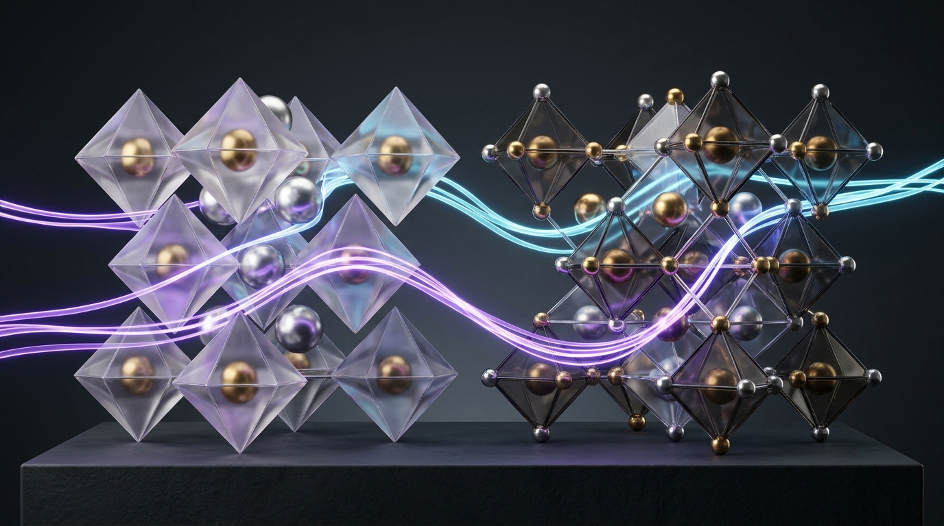
Até ao Capítulo 21, quase toda a nossa viagem focou-se em moléculas discretas descritas por conjuntos de base de Orbitais Gaussianas centradas nos núcleos (def2-TZVP, cc-pVTZ) e pela equação de Schrödinger não-relativista. Mas o mundo real da Química tem três grandes fronteiras onde esse paradigma precisa de ser ampliado: (1) E se o nosso sistema for um cristal periódico infinito, um semicondutor de baterias ou uma superfície metálica de platina \(\text{Pt}(111)\) em catálise heterogénea? (2) E se o nosso catalisador contiver metais pesados da 2.ª e 3.ª séries de transição ou lantanídeos/actinídeos (\(\text{Pd}, \text{Pt}, \text{Au}, \text{Hg}, \text{Pb}, \text{U}\)) onde os eletrões internos viajam a mais de metade da velocidade da luz? (3) E se precisarmos de ver moléculas de água e iões a moverem-se no tempo a \(300\text{ K}\) (Dinâmica Molecular Ab Initio, AIMD)? Neste Capítulo 22 vamos dominar estas três fronteiras de forma cristalina!
Up through Chapter 21, nearly our entire journey focused on discrete molecules described by atom-centered Gaussian basis sets (def2-TZVP, cc-pVTZ) and the non-relativistic Schrödinger equation. Yet the real world of Chemistry has three major frontiers where that paradigm must be expanded: (1) What if our system is an infinite periodic crystal, a battery semiconductor, or a catalytic \(\text{Pt}(111)\) metal surface? (2) What if our catalyst contains heavy 4d/5d transition metals or lanthanides/actinides (\(\text{Pd}, \text{Pt}, \text{Au}, \text{Hg}, \text{Pb}, \text{U}\)) whose inner electrons travel at over half the speed of light? (3) What if we need to watch liquid water and ions move in real time at \(300\text{ K}\) (Ab Initio Molecular Dynamics, AIMD)? In Chapter 22 we master all three frontiers!
22.1 De Moléculas a Cristais Periódicos: Teorema de Bloch, Zona de Brillouin (\(\mathbf{k}\)) e Energia de Corte de Ondas Planas (\(E_{\text{cut}}\)) 22.1 From Molecules to Periodic Crystals: Bloch's Theorem, Brillouin Zone (\(\mathbf{k}\)) & Plane-Wave Cutoff Energy (\(E_{\text{cut}}\))
Como é que um computador com memória finita consegue calcular as orbitais de um cristal macroscópico de sal (\(\text{NaCl}\)), de silício ou de uma superfície catalítica de \(\text{Pt}(111)\) que contém \(10^{23}\) átomos? Imagine que quer imprimir um papel de parede ou azulejar uma parede infinita: não precisa de desenhar milhões de metros de parede; basta desenhar um único azulejo unitário (a Célula Unitária, de vetores \(\mathbf{a}_1, \mathbf{a}_2, \mathbf{a}_3\)) e especificar a regra de repetição nas bordas! Em 1928, Felix Bloch provou que num potencial cristalino periódico \(V(\mathbf{r} + \mathbf{R}) = V(\mathbf{r})\), qualquer orbital eletrónica de todo o cristal é simplesmente uma função com a periodicidade de um único azulejo (\(u_{n\mathbf{k}}(\mathbf{r})\)) multiplicada por uma onda de fase suave \(e^{i\mathbf{k}\cdot\mathbf{r}}\)! How can a finite computer calculate the orbitals of a macroscopic crystal of table salt (\(\text{NaCl}\)), silicon, or a \(\text{Pt}(111)\) catalytic surface containing \(10^{23}\) atoms? Imagine designing wallpaper or tiling an infinite bathroom wall: you don't need to draw millions of square meters of wall; you only need to draw one single repeating tile (the Unit Cell, with lattice vectors \(\mathbf{a}_1, \mathbf{a}_2, \mathbf{a}_3\)) and specify how the pattern connects across the tile edges! In 1928, Felix Bloch proved that inside a periodic crystal potential \(V(\mathbf{r} + \mathbf{R}) = V(\mathbf{r})\), every electronic orbital of the entire crystal is simply a tile-periodic function \(u_{n\mathbf{k}}(\mathbf{r})\) multiplied by a smooth phase wave \(e^{i\mathbf{k}\cdot\mathbf{r}}\)!
Graças ao Teorema de Bloch, trocamos um problema impossível com \(10^{23}\) eletrões por um problema pequeno dentro de uma única célula unitária resolvido para uma grelha de vetores de onda \(\mathbf{k}\) (momento cristalino) na Primeira Zona de Brillouin do espaço recíproco (tipicamente uma grelha uniforme de Monkhorst–Pack, como \(6\times 6\times 6\) pontos \(\mathbf{k}\)). Thanks to Bloch's Theorem, we trade an impossible \(10^{23}\)-electron problem for a compact problem inside a single unit cell solved across a grid of wavevectors \(\mathbf{k}\) (crystal momentum) inside the First Brillouin Zone of reciprocal space (typically a uniform Monkhorst–Pack grid, such as \(6\times 6\times 6\) \(\mathbf{k}\)-points).
E qual é a forma mais natural de expandir uma função periódica \(u_{n\mathbf{k}}(\mathbf{r})\) dentro da célula unitária em programas de estado sólido como VASP, Quantum ESPRESSO ou CP2K? Uma série de Fourier de Ondas Planas \(e^{i(\mathbf{k}+\mathbf{G})\cdot\mathbf{r}}\), onde incluímos todos os vetores da rede recíproca \(\mathbf{G}\) cuja energia cinética não ultrapasse um único parâmetro de controlo: a Energia de Corte (\(E_{\text{cut}}\), em \(\text{eV}\) ou \(\text{Ry}\))!
And what is the most natural way to expand a periodic function \(u_{n\mathbf{k}}(\mathbf{r})\) inside the unit cell in solid-state codes such as VASP, Quantum ESPRESSO, or CP2K? A Fourier series of Plane Waves \(e^{i(\mathbf{k}+\mathbf{G})\cdot\mathbf{r}}\), retaining all reciprocal lattice vectors \(\mathbf{G}\) whose kinetic energy lies below a single control knob: the Cutoff Energy (\(E_{\text{cut}}\), in \(\text{eV}\) or \(\text{Ry}\))!
1. Um único botão para convergir a base (\(E_{\text{cut}}\)): Ao contrário das bases Gaussianas (onde temos dezenas de famílias
def2-SVP, cc-pVTZ, etc.), nas ondas planas basta aumentar um único número (\(E_{\text{cut}}\), tipicamente \(400\text{ a }600\text{ eV}\) no VASP) para tornar a base sistematicamente mais completa em todo o espaço!2. Regra de Ouro da Amostragem de Pontos \(\mathbf{k}\): Como o espaço recíproco é o inverso do espaço real, uma célula unitária pequena no espaço real exige muitos pontos \(\mathbf{k}\) (ex.: \(12\times 12\times 12\) para um cristal metálico pequeno de \(\text{Cu}\), porque os metais têm uma superfície de Fermi descontínua), enquanto uma supercélula grande (\(> 15\text{ Å}\)) ou uma molécula isolada numa caixa exige apenas um único ponto: o Ponto Gama (\(\Gamma, \mathbf{k} = \mathbf{0}\))! 1. A single knob for basis-set convergence (\(E_{\text{cut}}\)): Unlike Gaussian basis sets (where we juggle dozens of families like
def2-SVP, cc-pVTZ, etc.), with plane waves you simply turn up one single number (\(E_{\text{cut}}\), typically \(400\text{–}600\text{ eV}\) in VASP) to approach the Complete Basis Set limit smoothly everywhere in space!2. Golden Rule of \(\mathbf{k}\)-Point Sampling: Because reciprocal space is the inverse of real space, a small unit cell in real space requires a dense \(\mathbf{k}\)-point mesh (e.g., \(12\times 12\times 12\) for bulk metallic \(\text{Cu}\), since metals have a sharp Fermi surface), whereas a large supercell (\(> 15\text{ Å}\)) or a molecule in a box requires only a single point: the Gamma Point (\(\Gamma, \mathbf{k} = \mathbf{0}\))!
22.2 Porque é que as Ondas Planas Não Têm BSSE nem Forças de Pulay? O Método PAW de Blöchl
22.2 Why Do Plane Waves Have Zero BSSE and Zero Pulay Forces? Blöchl's PAW Method
Quando estudámos bases Gaussianas centradas nos núcleos (Bloco III), vimos dois problemas inevitáveis pelo facto de cada função de base \(\chi_\mu(\mathbf{r} - \mathbf{R}_A)\) «viajar agarrada às costas do seu núcleo \(\mathbf{R}_A\)»: (1) quando uma molécula \(A\) se aproxima de uma superfície ou de outra molécula \(B\), «pede emprestadas» funções de base do vizinho, criando uma atração artificial espúria chamada Erro de Sobreposição do Conjunto de Base (BSSE); e (2) quando calculamos forças atómicas \(-\partial E / \partial \mathbf{R}_A\) para otimizar uma geometria, temos de calcular derivadas das próprias funções de base (as Forças de Pulay).
When we studied atom-centered Gaussian basis sets (Block III), we encountered two unavoidable side effects of having each basis function \(\chi_\mu(\mathbf{r} - \mathbf{R}_A)\) "ride on the back of its nucleus \(\mathbf{R}_A\)": (1) when molecule \(A\) approaches a surface or another molecule \(B\), it "borrows" basis functions from its neighbor, creating a spurious artificial attraction called Basis Set Superposition Error (BSSE); and (2) when evaluating atomic forces \(-\partial E / \partial \mathbf{R}_A\) for geometry optimization, we must compute derivatives of the moving basis functions themselves (Pulay Forces).
Pode: coloca-se a molécula numa caixa periódica grande, com vácuo suficiente (tipicamente 10 a 15 Å) para que as cópias vizinhas não interajam. Mas é pouco eficiente: as ondas planas preenchem uniformemente toda a caixa, incluindo o vácuo, e as moléculas carregadas exigem correções especiais. Para moléculas, as funções gaussianas centradas nos átomos são muito mais económicas. As ondas planas brilham em sólidos, superfícies e líquidos periódicos, onde os átomos ocupam todo o espaço.You can: the molecule is placed in a large periodic box, with enough vacuum (typically 10 to 15 Å) that neighboring copies do not interact. But it is inefficient: plane waves fill the entire box uniformly, including the vacuum, and charged molecules need special corrections. For molecules, atom-centered Gaussian functions are much cheaper. Plane waves shine for solids, surfaces, and periodic liquids, where atoms fill all of space.
Ora, as ondas planas \(e^{i(\mathbf{k}+\mathbf{G})\cdot\mathbf{r}}\) não dependem da posição de nenhum átomo \(\mathbf{R}_A\) — preenchem toda a caixa de forma perfeitamente uniforme e democrática! Por isso, num cálculo de ondas planas, o erro BSSE é rigorosamente zero (\(\text{BSSE} = 0\)) (ideal para calcular energias de adsorção de gases em catalisadores heterogéneos!) e as forças de Pulay são rigorosamente nulas. Em contrapartida, como as orbitais de valência oscilam muito rapidamente perto dos núcleos (para serem ortogonais aos eletrões do caroço \(1s, 2s, 2p\)), descrever todos os eletrões com ondas planas exigiria um corte absurdo (\(E_{\text{cut}} > 50\,000\text{ eV}\)). A solução moderna nos códigos periódicos é o método PAW (Projector-Augmented Wave, Peter Blöchl, 1994) ou a abordagem mista Gaussiana + Ondas Planas (GPW no CP2K):
Plane waves \(e^{i(\mathbf{k}+\mathbf{G})\cdot\mathbf{r}}\), by contrast, do not depend on any nuclear position \(\mathbf{R}_A\) — they fill the entire simulation box uniformly and democratically! Consequently, in a plane-wave calculation, BSSE is strictly zero (\(\text{BSSE} = 0\)) (making plane waves ideal for computing gas adsorption energies on heterogeneous catalysts!) and Pulay forces vanish identically. Conversely, because valence orbitals oscillate violently near the nuclei (to stay orthogonal to the \(1s, 2s, 2p\) core shells), describing all electrons directly with plane waves would demand an absurd cutoff (\(E_{\text{cut}} > 50\,000\text{ eV}\)). The modern solution in periodic codes is Blöchl's Projector-Augmented Wave (PAW, 1994) method or the mixed Gaussian and Plane Waves scheme (GPW in CP2K):
PAW DE BLÖCHL: DA FUNÇÃO DE ONDA SUAVE \(\tilde{\Psi}_n\) À FUNÇÃO DE ONDA REAL DE TODOS OS ELETRÕES \(\Psi_n\)BLÖCHL'S LINEAR PAW TRANSFORMATION: FROM SMOOTH PSEUDO-WAVEFUNCTION \(\tilde{\Psi}_n\) TO ALL-ELECTRON WAVEFUNCTION \(\Psi_n\)
Usamos o chamado Modelo de Placa com Vácuo (Periodic Slab Model)! Construímos uma caixa periódica com \(4\text{ a }6\) camadas atómicas de \(\text{Pt}(111)\) que se repetem infinitamente nas direções laterais \(x\) e \(y\), mas adicionamos \(15\text{ a }20\text{ Å}\) de espaço vazio (vácuo) na direção vertical \(z\) por cima da molécula adsorvida (juntamente com uma correção de dipolo em \(z\)). Assim, o topo da nossa placa catalítica nunca «sente» a base da imagem periódica seguinte no eixo \(z\)! (A única desvantagem das ondas planas é que esse espaço vazio em \(z\) também tem de ser preenchido com ondas planas — razão pela qual para moléculas isoladas no vácuo as bases Gaussianas no ORCA são muito mais rápidas do que ondas planas!). We use the Periodic Slab Model! We build a periodic supercell containing \(4\text{–}6\) atomic layers of \(\text{Pt}(111)\) that repeat infinitely along the lateral \(x\) and \(y\) directions, while inserting \(15\text{–}20\text{ Å}\) of empty vacuum along the vertical \(z\) axis above the adsorbed molecule (together with a \(z\)-dipole correction). That way, the top of our catalytic slab never interacts with the bottom of the next periodic image along \(z\)! (The only drawback of plane waves is that empty vacuum still requires plane-wave grid points — which is why atom-centered Gaussians in ORCA are much faster than plane waves for isolated gas-phase molecules!).
22.3 Química Quântica Relativista: Porque é que o Ouro é Amarelo, o Mercúrio é Líquido e Como Funcionam ECP, ZORA e DKH2?
22.3 Relativistic Quantum Chemistry: Why Is Gold Yellow, Why Is Mercury Liquid & How Do ECP, ZORA, and DKH2 Work?
Costuma ouvir-se dizer que a Teoria da Relatividade Restrita de Einstein (1905) só interessa a astrofísicos ou físicos de partículas, e nunca à Química. Nada podia estar mais longe da verdade! Em unidades atómicas, a velocidade da luz é \(c \approx 137.036\text{ a.u.}\) (\(\alpha = 1/c \approx 1/137\) é a constante de estrutura fina), e a velocidade média de um eletrão \(1s\) num átomo de número atómico \(Z\) é \(v_{1s} \approx Z\text{ a.u.}\), ou seja, \(\mathbf{v_{1s}/c \approx Z/137}\)! People often assume Einstein's Special Theory of Relativity (1905) only matters to astrophysicists or particle physicists, never to chemists. Nothing could be further from the truth! In atomic units, the speed of light is \(c \approx 137.036\text{ a.u.}\) (\(\alpha = 1/c \approx 1/137\) is the fine-structure constant), and the average speed of a \(1s\) electron in an atom of atomic number \(Z\) is \(v_{1s} \approx Z\text{ a.u.}\), meaning \(\mathbf{v_{1s}/c \approx Z/137}\)!
No ouro (\(Z = 79\)), os eletrões \(1s\) movem-se a cerca de 58% da velocidade da luz (aproximadamente \(Z/137\) em unidades atómicas). Pela relatividade, isso aumenta a sua massa efetiva em cerca de 20%, e um eletrão mais pesado orbita mais perto do núcleo. Imagine um corredor numa pista circular que fica mais pesado à medida que acelera e é puxado para a pista interior. Todas as orbitais \(s\) do ouro contraem-se, incluindo a \(6s\), e as orbitais \(5d\), mais blindadas, expandem-se. O espaço de energia entre \(5d\) e \(6s\) diminui o suficiente para o ouro absorver luz azul, e por isso vemos a cor complementar: amarelo. Sem relatividade, o ouro seria prateado como a prata.In gold (\(Z = 79\)), the \(1s\) electrons move at about 58% of the speed of light (roughly \(Z/137\) in atomic units). By relativity, that raises their effective mass by about 20%, and a heavier electron orbits closer to the nucleus. Picture a runner on a circular track who gets heavier as he speeds up and is pulled toward the inside lane. All of gold's \(s\) orbitals contract, including \(6s\), while the more shielded \(5d\) orbitals expand. The energy gap between \(5d\) and \(6s\) shrinks enough for gold to absorb blue light, so we see the complementary color: yellow. Without relativity, gold would be silvery like silver.
Para o Carbono (\(Z = 6\)), \(v_{1s}/c \approx 4.4\%\), e o efeito relativista é minúsculo. Mas para o Ouro (\(\text{Au}, Z = 79\)) ou o Mercúrio (\(\text{Hg}, Z = 80\)), os eletrões \(1s\) viajam a \(\mathbf{79/137 \approx 58\%}\) da velocidade da luz! A essa velocidade, a Equação de Dirac de 4 componentes (ou as suas reduções de 2/1 componentes para químicos) produz três consequências químicas profundas que mudam a Tabela Periódica a partir do 4.º e 5.º períodos: For Carbon (\(Z = 6\)), \(v_{1s}/c \approx 4.4\%\), and relativistic effects are tiny. Yet for Gold (\(\text{Au}, Z = 79\)) or Mercury (\(\text{Hg}, Z = 80\)), the \(1s\) electrons travel at \(\mathbf{79/137 \approx 58\%}\) of the speed of light! At such speeds, Dirac's 4-component equation (and its 2/1-component reductions for chemists) produces three profound chemical effects that reshape the Periodic Table from the 4th and 5th rows onward:
ZORARELATIVISTIC ELECTRON MASS \(m_{\text{rel}}\), BOHR RADIUS CONTRACTION \(a_{\text{rel}}\) & SCALAR ZORA EQUATION
2. Porque é que a Prata (\(\text{Ag}, Z=47\)) é branca/espelhada mas o Ouro (\(\text{Au}, Z=79\)) é amarelo-dourado? Num cálculo de Schrödinger não-relativista, o Ouro teria exatamente a mesma cor prateada da Prata (a transição eletrónica da banda \(5d\) cheia para a banda de condução \(6s\) estaria no Ultravioleta, a \(\sim 3.6\text{ eV}\))! Mas com a relatividade, a orbital \(6s\) do Ouro desce e a banda \(5d\) sobe, estreitando o hiato \(5d \to 6s\) para \(\mathbf{2.4\text{ eV}}\) (\(\lambda \approx 515\text{ nm}\)): o Ouro absorve a luz azul/violeta do espectro visível e reflete o amarelo/vermelho! E é também a forte contração da orbital \(6s^1\) que torna o Ouro nobre e permite ligações curtíssimas \(\text{Au–Au}\) (interações aurofílicas)!
3. Porque é que o Mercúrio (\(\text{Hg}, Z=80, [\text{Xe}]4f^{14}5d^{10}6s^2\)) é o único metal líquido à temperatura ambiente (\(T_{\text{fusão}} = -39^\circ\text{C}\))? No \(\text{Hg}\), a subcamada \(6s^2\) totalmente preenchida está tão fortemente contraída e estabilizada pela relatividade (efeito do par inerte relativista) que os átomos de \(\text{Hg}\) recusam partilhar os eletrões \(6s^2\) para formar ligações metálicas fortes, comportando-se quase como um «gás nobre pesado» (como o Xénon)! Pela mesma razão no Chumbo (\(\text{Pb}, Z=82\)), o par \(6s^2\) é tão estável que o \(\text{PbO}_2\) (\(\text{Pb}^{\text{IV}}\)) quer desesperadamente receber \(2\) eletrões para regressar a \(\text{Pb}^{\text{II}}\) (\(6s^2\)) — gerando cerca de \(1.7\text{ dos }2.1\text{ Volts}\) de cada célula da bateria de chumbo-ácido de \(12\text{ V}\) que põe o seu carro a trabalhar todas as manhãs! 1. Direct Relativistic Contraction of \(s\) (and \(p_{1/2}\)) Orbitals vs. Indirect Expansion of \(d\) and \(f\) Orbitals: Because \(s\) orbitals penetrate right to the nucleus where speeds approach \(c\), the relativistic mass increase \(m_{\text{rel}}\) causes all \(1s, 2s, \dots, 6s\) orbitals to contract and drop strongly in energy! Conversely, because those contracted \(s\) shells screen the nuclear charge more effectively, the \(4d, 5d\) and \(4f, 5f\) orbitals (which have nodes at the nucleus) feel weaker nuclear attraction and expand radially and rise in energy!
2. Why is Silver (\(\text{Ag}, Z=47\)) white/mirror-like while Gold (\(\text{Au}, Z=79\)) is yellow? In a non-relativistic Schrödinger calculation, Gold would look just as silvery-white as Silver (its \(5d \to 6s\) interband transition would lie in the Ultraviolet at \(\sim 3.6\text{ eV}\))! With relativity turned on, Gold's \(6s\) orbital drops and its \(5d\) band rises, narrowing the \(5d \to 6s\) gap to \(\mathbf{2.4\text{ eV}}\) (\(\lambda \approx 515\text{ nm}\)): Gold absorbs blue/violet visible light and reflects yellow/red! That same \(6s^1\) contraction also makes Gold noble and drives short \(\text{Au–Au}\) aurophilic interactions!
3. Why is Mercury (\(\text{Hg}, Z=80, [\text{Xe}]4f^{14}5d^{10}6s^2\)) the only metal that is liquid at room temperature (\(T_{\text{melt}} = -39^\circ\text{C}\))? In \(\text{Hg}\), the filled \(6s^2\) subshell is so tightly contracted and stabilized by relativity (the relativistic inert-pair effect) that \(\text{Hg}\) atoms refuse to share their \(6s^2\) electrons into strong metallic bands, behaving almost like a heavy noble gas (like Xenon)! By the exact same mechanism in Lead (\(\text{Pb}, Z=82\)), the \(6s^2\) pair is so stable that \(\text{PbO}_2\) (\(\text{Pb}^{\text{IV}}\)) eagerly pulls in \(2\) electrons to revert to \(\text{Pb}^{\text{II}}\) (\(6s^2\)) — generating roughly \(1.7\text{ of the }2.1\text{ Volts}\) per cell in the \(12\text{ V}\) lead-acid battery that starts your car every morning!
def2-ECP vs. ZORA / DKH2 no ORCA?Practical Lab Rule: When to Use def2-ECP vs. ZORA / DKH2 in ORCA?• Para geometrias, barreiras e termoquímica de rotina com metais pesados (\(Z \ge 37\), de \(\text{Rb}, \text{Pd}, \text{Ag}\) até \(\text{Pt}, \text{Au}, \text{Hg}, \text{Pb}\)): Basta pedir qualquer base da família
def2-SVP, def2-TZVP ou def2-QZVP no ORCA! O programa substitui automaticamente os eletrões internos por Potenciais Efetivos de Caroço Relativistas de Estugarda–Colónia (def2-ECP) que já incorporam a contração relativista escalar sem custo extra!• Para propriedades que dependem da densidade eletrónica perto do núcleo (RMN de metais pesados, EPR, espetroscopia de raios X / Mössbauer ou Acoplamento Spin–Órbita
SOC): Aqui não podemos apagar o caroço com um ECP! Temos de fazer um cálculo relativista de todos os eletrões (! ZORA, ! DKH2 ou ! X2C) acompanhado obrigatoriamente por conjuntos de base recontraídos para relatividade: ZORA-def2-TZVP ou DKH-def2-TZVP para elementos até \(Z=36\) e SARC-ZORA-TZVP / SARC-DKH-TZVP (de Pantazis e Neese) ou x2c-TZVPall para elementos pesados (\(Z > 36\))!
• For routine geometries, barriers, and thermochemistry with heavy elements (\(Z \ge 37\), from \(\text{Rb}, \text{Pd}, \text{Ag}\) to \(\text{Pt}, \text{Au}, \text{Hg}, \text{Pb}\)): Simply request any basis set from the def2-SVP, def2-TZVP, or def2-QZVP family in ORCA! The code automatically replaces the inner core shells with Stuttgart–Cologne Relativistic Effective Core Potentials (def2-ECP) that build scalar relativistic contraction right in at reduced cost!• For core-sensitive properties (heavy-element NMR, EPR, X-ray / Mössbauer spectroscopy, or Spin–Orbit Coupling
SOC): Here we cannot replace the core with an ECP! We must run an all-electron relativistic Hamiltonian (! ZORA, ! DKH2, or ! X2C) paired strictly with relativistically recontracted basis sets: ZORA-def2-TZVP or DKH-def2-TZVP up to \(Z=36\) and SARC-ZORA-TZVP / SARC-DKH-TZVP (by Pantazis & Neese) or x2c-TZVPall for heavy elements (\(Z > 36\))!
22.4 Dinâmica Molecular Ab Initio (BOMD vs. CPMD) e Amostragem de Eventos Raros (Metadinâmica e Umbrella Sampling)
22.4 Ab Initio Molecular Dynamics (BOMD vs. CPMD) & Rare-Event Sampling (Metadynamics & Umbrella Sampling)
Nos Capítulos 18 a 21 estudámos a superfície de energia potencial através de pontos estacionários estáticos (mínimos e estados de transição). Mas em líquidos estruturados (como a transferência de um protão \(\text{H}^+\) através da rede de pontes de hidrogénio da água pelo mecanismo de Grotthuss, ou eletrólitos concentrados na interface de uma bateria), não existe um único mínimo isolado: o solvente reorganiza-se continuamente à temperatura \(T\)! Na Dinâmica Molecular Ab Initio (AIMD), integramos as equações de movimento de Newton para os núcleos (\(M_A \ddot{\mathbf{R}}_A = -\nabla_A E_{\text{QM}}\)) em passos de tempo de \(\Delta t \approx 0.5\text{ a }1.0\text{ fs}\), calculando as forças em cada instante diretamente por DFT («em voo», sem campos de forças clássicos parametrizados!).
In Chapters 18–21 we explored the potential energy surface via static stationary points (minima and transition states). Yet in structured liquids (such as proton \(\text{H}^+\) hopping across liquid water's hydrogen-bond network via the Grotthuss mechanism, or concentrated electrolytes at a battery electrode interface), there is no single isolated minimum: the solvent reorganizes continuously at temperature \(T\)! In Ab Initio Molecular Dynamics (AIMD), we integrate Newton's equations of motion for the nuclei (\(M_A \ddot{\mathbf{R}}_A = -\nabla_A E_{\text{QM}}\)) in time steps of \(\Delta t \approx 0.5\text{–}1.0\text{ fs}\), computing the forces on the fly directly from DFT (with no parameterized classical force fields!).
Os protões movem-se na água muito mais depressa do que outros iões do mesmo tamanho. A dinâmica molecular ab initio mostrou porquê: o protão não viaja sozinho. Em vez disso, as ligações O–H e as pontes de hidrogénio reorganizam-se em cadeia, e uma molécula de água passa um protão à vizinha, que passa outro à seguinte, como numa fila de pessoas a passar baldes. Este mecanismo, proposto por Grotthuss em 1806, só pôde ser observado em detalhe com simulações em que as ligações se formam e quebram, o que um campo de forças clássico não permite. É também o mecanismo do transporte de protões em muitas enzimas e em membranas de células de combustível.Protons move through water much faster than other ions of the same size. Ab initio molecular dynamics showed why: the proton does not travel alone. Instead, the O–H bonds and hydrogen bonds rearrange in a chain, and one water molecule hands a proton to its neighbor, which hands another on to the next, like a line of people passing buckets. This mechanism, proposed by Grotthuss in 1806, could only be observed in detail with simulations in which bonds form and break, which a classical force field does not allow. It is also the mechanism of proton transport in many enzymes and in fuel-cell membranes.
Existem duas grandes famílias de AIMD — a Dinâmica de Born–Oppenheimer (BOMD) (que converge o ciclo SCF eletrónico em cada passo de tempo de \(0.5\text{ fs}\)) e a Dinâmica de Car–Parrinello (CPMD, 1985) (que atribui uma massa fictícia pequena \(\mu\) às orbitais de Kohn–Sham para evoluírem classicamente ao lado dos núcleos sem repetir ciclos SCF) —, combinadas com técnicas de Amostragem Avançada (Metadinâmica de Parrinello/Laio ou Umbrella Sampling) para vencer barreiras químicas altas:
There are two major families of AIMD — Born–Oppenheimer MD (BOMD) (which fully converges the electronic SCF cycle at every \(0.5\text{ fs}\) time step) and Car–Parrinello MD (CPMD, 1985) (which assigns a small fictitious mass \(\mu\) to the Kohn–Sham orbitals so they propagate smoothly alongside the nuclei without re-solving the SCF at every step) — combined with Enhanced Sampling (Parrinello/Laio's Metadynamics or Umbrella Sampling) to cross high chemical barriers:
BOMD), LAGRANGIANO DE CAR–PARRINELLO (CPMD) E METADINÂMICABORN–OPPENHEIMER EQUATIONS OF MOTION (BOMD), CAR–PARRINELLO LAGRANGIAN (CPMD) & METADYNAMICS BIAS
$$\begin{gathered} M_A\frac{d^2\mathbf{R}_A}{dt^2} = -\nabla_{\mathbf{R}_A}\min_{\{\psi_i\}} E_{\text{KS}}\bigl[\{\psi_i\};\mathbf{R}\bigr] \quad (\text{BOMD}), \qquad \mathcal{L}_{\text{CPMD}} = \sum_A \frac{1}{2}M_A\dot{\mathbf{R}}_A^2 + \sum_i \frac{1}{2}\mu\langle\dot{\psi}_i|\dot{\psi}_i\rangle - E_{\text{KS}} + \sum_{ij}\Lambda_{ij}\bigl(\langle\psi_i|\psi_j\rangle - \delta_{ij}\bigr) \\[6pt] V_{\text{bias}}^{\text{MetaD}}\bigl(\mathbf{s}, t\bigr) = \sum_{t' < t} W \exp\!\left(-\frac{\bigl|\mathbf{s}(\mathbf{R}) - \mathbf{s}(t')\bigr|^2}{2\sigma_s^2}\right) \xrightarrow{t\to\infty} -F(\mathbf{s}) + C \end{gathered}$$
Uma trajetória
AIMD normal dura apenas \(20\text{ a }100\text{ ps}\) (\(10^{-10}\text{ s}\)). Se uma reação química tiver uma barreira \(\Delta G^\ddagger = 15\text{ kcal/mol}\), à temperatura ambiente ela só acontece uma vez a cada milissegundo (\(10^{-3}\text{ s}\)) — teríamos de esperar dez milhões de vezes mais tempo do que a simulação dura! Na Metadinâmica, escolhemos uma variável coletiva \(\mathbf{s}(\mathbf{R})\) (por exemplo, a diferença de distâncias das ligações que quebram e formam) e, a cada poucos passos, o computador «deita um pequeno monte de areia Gaussiano» \(V_{\text{bias}}\) no sítio onde a molécula está. Pouco a pouco, a areia enche o poço dos reagentes até a molécula ser empurrada por cima do Estado de Transição! No fim, a quantidade de areia acumulada dá-nos o perfil completo da Energia Livre de Helmholtz/Gibbs \(F(\mathbf{s}) = -V_{\text{bias}}(\mathbf{s})\)!
An unbiased AIMD trajectory typically spans only \(20\text{–}100\text{ ps}\) (\(10^{-10}\text{ s}\)). If a chemical reaction has a barrier of \(\Delta G^\ddagger = 15\text{ kcal/mol}\), at room temperature a reactive event happens only once every millisecond (\(10^{-3}\text{ s}\)) — ten million times longer than our entire simulation! In Metadynamics, we pick a collective variable \(\mathbf{s}(\mathbf{R})\) (such as the difference between breaking and forming bond lengths) and every few steps the computer "drops a small Gaussian pile of sand" \(V_{\text{bias}}\) wherever the system currently sits. Gradually, the sand fills up the reactant basin until the molecule is pushed right over the Transition State! At the end, the negative of the accumulated sand pile gives the exact Free-Energy surface \(F(\mathbf{s}) = -V_{\text{bias}}(\mathbf{s})\)!
Objetivo: Quantificar os efeitos relativistas ao longo da Tabela Periódica (velocidade \(v_{1s}/c \approx Z/137\) e contração relativista das orbitais \(s\)) e escolher o protocolo adequado (pseudopotenciais ECP vs. ZORA/DKH2 e energia de corte \(E_{\text{cut}}\) em sólidos periódicos, Capítulo 22). Goal: Quantify relativistic effects across the Periodic Table (speed \(v_{1s}/c \approx Z/137\) and relativistic \(s\)-orbital contraction) and select the proper computational setup (ECP pseudopotentials vs. ZORA/DKH2 and plane-wave cutoff \(E_{\text{cut}}\) in periodic solids, Chapter 22).
ℹ️ Explicação deste seletor / controlo (clique para abrir)ℹ️ Explanation of this selector / control (click to open)
O que observar: Mostra a velocidade relativista do eletrão \(1s\) (\(v_{1s}/c \approx Z/137\)), a contração relativista das orbitais \(s/p\) (que explica a cor amarela do Ouro \(Z=79\) e o estado líquido do Mercúrio \(Z=80\)) e quando é obrigatório usar ECPs ou ZORA/DKH2.What it controls: Selects the atomic number \(Z\) across the Periodic Table.
What to observe: Displays the \(1s\) electron relativistic speed (\(v_{1s}/c \approx Z/137\)), the relativistic contraction of \(s/p\) orbitals (explaining the yellow color of Gold \(Z=79\) and liquid state of Mercury \(Z=80\)), and when ECPs or ZORA/DKH2 are mandatory.
ℹ️ Explicação deste seletor / controlo (clique para abrir)ℹ️ Explanation of this selector / control (click to open)
Questões acessíveis sobre os conceitos essenciais deste capítulo • Clique em «Outra Variante» ou «Feedback de Estudo» para saber o que estudar mais.Accessible questions on this chapter's essential concepts • Click "Swap Variant" or "Study Feedback" for personalized study guidance.
Ao longo de 22 capítulos reunimos um arsenal impressionante de métodos quânticos: Hartree–Fock, MP2, CCSD(T), CASSCF, funcionais DFT da Escada de Jacob, bases Gaussianas e de ondas planas, correções de dispersão D3/D4, relatividade, solvatação SMD e termoquímica qRRHO. Mas quando um estudante se senta diante do computador para começar a sua tese, surge a dúvida mais importante de todas: «Como escolho uma combinação equilibrada de método, base e modelo ambiental sem cair em cancelamentos de erros enganadores, e como defendo as minhas escolhas perante os revisores de uma revista científica?» É esse guia forense que vamos construir no Capítulo 23! Across 22 chapters we have assembled an impressive arsenal of quantum methods: Hartree–Fock, MP2, CCSD(T), CASSCF, Jacob's Ladder DFT functionals, Gaussian and plane-wave basis sets, D3/D4 dispersion, relativity, SMD solvation, and qRRHO thermochemistry. Yet when a student sits down at the computer to start a thesis project, the most important question of all arises: "How do I choose a balanced combination of method, basis set, and environment model without falling into fortuitous error cancellation, and how do I defend my protocol to journal referees?" That forensic survival guide is the subject of Chapter 23!
📘 Conceito Principal Explicado: Dualidade Onda–Partícula, Efeito Fotoelétrico e Confinamento QuânticoCore Concept Explained: Wave–Particle Duality, the Photoelectric Effect, and Quantum Confinement
Porque é que uma luz vermelha intensíssima não arranca um único eletrão de uma placa de potássio, enquanto uma luz ultravioleta muito fraca arranca eletrões instantaneamente? Porque o efeito fotoelétrico não é uma 'onda contínua a aquecer a superfície', mas sim uma colisão individual $1:1$ entre um fotão de energia $h\nu$ e um eletrão preso pela função trabalho $\Phi$ (energia de ionização): Why does intense red light fail to eject electrons from potassium metal while faint UV light ejects them immediately? Because photoemission is a $1:1$ collision between a single photon of energy $h\nu$ and an electron bound by work function $\Phi$:
💡 Intuição Física:Physical Intuition: Repare como $\lambda = h/p$ explica imediatamente a quantização na caixa de tamanho $L$: para a onda do eletrão não se anular nas paredes, têm de caber meias-ondas inteiras ($L = n\,\lambda/2$), o que força a energia a saltar em degraus discretos $E_n \propto n^2/L^2$! Notice how $\lambda = h/p$ explains quantization in a box of length $L$: standing waves require $L = n\lambda/2$, forcing energy into discrete steps $E_n \propto n^2/L^2$!
🌍 Curiosidade & Ligação ao Mundo Real: Porque é que as cenouras são cor de laranja e os Pontos Quânticos (Nobel 2023) brilham em todas as cores?Curiosity & Real-World Connection: Why are carrots orange and why do Quantum Dots (Nobel 2023) glow in every color of the rainbow?
A fórmula da partícula na caixa ($\Delta E \propto 1/L^2$) está nos seus olhos neste preciso momento! No $\beta$-caroteno da cenoura, os $22$ eletrões $\pi$ conjugados movem-se ao longo de uma 'caixa molecular 1D' de $L \approx 20\text{ Å}$, cujo salto quântico HOMO$\rightarrow$LUMO absorve luz azul-esverdeada ($\sim 450\text{ nm}$), refletindo o laranja complementar. E nos televisores QLED modernos (Pontos Quânticos, Prémio Nobel da Química 2023 para Bawendi, Brus e Ekimov), nanocristais do mesmo semicondutor ($\text{CdSe}$ ou $\text{InP}$) emitem luz vermelha quando têm $6\text{ nm}$ ($L$ grande $\Rightarrow \Delta E$ pequeno) e luz azul quando têm $2\text{ nm}$ ($L$ pequeno $\Rightarrow \Delta E$ grande)! The particle-in-a-box law ($\Delta E \propto 1/L^2$) explains why $\beta$-carotene's conjugated $\pi$-chain ($L\approx 20\text{ Å}$) absorbs blue light to make carrots look orange, and why semiconductor Quantum Dots (Nobel Prize 2023) emit red light at $6\text{ nm}$ diameter and blue light at $2\text{ nm}$!
🏛️ Mostrar Cientistas Pioneiros e Fotografias Históricas da Wikipedia relacionados com este Bloco (4 Cartões Ilustrados)Show Related Pioneer Scientists & Historical Wikipedia Photos (4 Illustrated Cards)
 Nobel 1918 • Constante de Planck hNobel 1918 • Planck's Constant h
Max Planck (1858–1947) ↗
Inaugurou a física quântica em 1900 ao demonstrar que a troca de energia entre matéria e radiação ocorre em pacotes discretos E = h*nu. Inaugurated quantum physics in 1900 by showing that energy exchange between matter and radiation occurs in discrete quanta E = h*nu.
 Nobel 1921 • Efeito Fotoelétrico & FotõesNobel 1921 • Photoelectric Effect & Photons
Albert Einstein (1879–1955) ↗
Demonstrou a natureza corpuscular dos quanta de luz (fotões, 1905) e a capacidade calorífica quântica dos sólidos vibracionais (1907). Demonstrated the particle nature of light quanta (photons, 1905) and the quantum heat capacity of vibrating solids (1907).
 Nobel 1929 • Ondas de Matéria (lambda = h/p)Nobel 1929 • Matter Waves (lambda = h/p)
Louis de Broglie (1892–1987) ↗
Unificou a dualidade onda-partícula para os eletrões, explicando fisicamente as órbitas estacionárias de Bohr como ondas construtivas. Unified wave-particle duality for electrons, physically explaining Bohr's stationary orbits as constructive standing waves.
 Nobel 1937 • Difração de Eletrões (1927)Nobel 1937 • Electron Diffraction (1927)
Clinton Davisson & G. P. Thomson ↗
Comprovaram experimentalmente a hipótese de de Broglie ao observar padrões de difração de Bragg quando feixes de eletrões atravessam cristais. Experimentally confirmed de Broglie's hypothesis by observing Bragg diffraction patterns when electron beams pass through crystals.
As 5 Fontes Ortogonais de Erro, Validação GMTKN55 (WTMAD-2) e Guia de Sobrevivência para Publicação
The 5 Orthogonal Error Sources, GMTKN55 (WTMAD-2) Validation & Publication Survival Guide
Anatomia do erro computacional, porque é que o clássico B3LYP/6-31G* é um «Ponto de Pauling» obsoleto, a hierarquia moderna de 3 níveis (GFN2-xTB \(\to\) r2SCAN-3c \(\to\) ωB97M-V / DLPNO-CCSD(T)) e a Checklist de 7 Pontos antes de submeter um artigo
Anatomy of computational error, why classic B3LYP/6-31G* is an obsolete "Pauling Point", the modern 3-tier hierarchy (GFN2-xTB \(\to\) r2SCAN-3c \(\to\) ωB97M-V / DLPNO-CCSD(T)) & the 7-Point Pre-Submission Audit Checklist
Nenhum piloto de aviação comercial descola confiando apenas na memória: segue sempre uma lista de verificação sistemática para garantir que nenhum subsistema crítico foi esquecido. Na Química Quântica Moderna acontece exatamente o mesmo: um programa como o ORCA ou o Gaussian quase nunca «dá erro de sintaxe» quando escolhemos uma aproximação física inadequada — ele converge silenciosamente e imprime uma energia com 10 casas decimais que pode estar errada em \(15\text{ kcal/mol}\)! Neste Capítulo 23 vamos aprender a decompor qualquer cálculo nas suas 5 fontes independentes de erro, a consultar a maior base de dados de validação da história da Química (GMTKN55) e a aplicar a Checklist de Auditoria de 7 Pontos a todos os seus projetos.
No commercial airline pilot takes off relying on memory alone: they follow a systematic pre-flight checklist to ensure no critical subsystem was overlooked. In Modern Quantum Chemistry, the exact same principle applies: a program like ORCA or Gaussian rarely prints a syntax error when you pick an inappropriate physical approximation — it quietly converges and prints an energy to 10 decimal places that may be wrong by \(15\text{ kcal/mol}\)! In Chapter 23 we learn to decompose any calculation into its 5 orthogonal sources of error, read the largest validation benchmark in chemistry history (GMTKN55), and apply the 7-Point Audit Checklist to every research project.
23.1 As 5 Fontes Ortogonais de Erro num Cálculo Quântico e o Perigo de «Colocar Pneus de Fórmula 1 num Trator» 23.1 The 5 Orthogonal Error Sources in a Quantum Calculation & the Danger of "Putting Formula 1 Tires on a Tractor"
Imagine que quer bater um recorde de velocidade em pista: de que serve gastar uma fortuna a montar pneus de Fórmula 1 de última geração (um conjunto de base quádruplo-\(\zeta\) gigante def2-QZVP) num trator agrícola com motor a gasóleo antigo (um funcional sem dispersão ou Hartree–Fock)? Ou ao contrário: de que serve comprar um motor de Ferrari (CCSD(T)) e montá-lo com rodas de madeira (uma base mínima STO-3G ou 6-31G*)? O erro total do seu cálculo é sempre dominado pelo elo mais fraco da corrente!
Imagine trying to set a lap record on a race track: what good does it do to spend a fortune mounting state-of-the-art Formula 1 tires (a massive quadruple-\(\zeta\) def2-QZVP basis set) on an old diesel farm tractor (an uncorrected functional or Hartree–Fock)? Or conversely: what good is buying a Ferrari engine (CCSD(T)) and bolting it onto wooden wagon wheels (a tiny STO-3G or 6-31G* basis set)? The total error of your calculation is always dominated by the weakest link in the chain!
Para desenhar um protocolo computacional equilibrado e atingir a desejada «Precisão Química» (\(\pm 1.0\text{ kcal/mol}\)), devemos encarar a diferença entre a Energia Livre calculada \(\Delta G_{\text{calc}}^\circ\) e a experimental \(\Delta G_{\text{exp}}^\circ\) como a soma de cinco componentes de erro ortogonais (independentes entre si). To design a balanced computational protocol and achieve "Chemical Accuracy" (\(\pm 1.0\text{ kcal/mol}\)), we must view the discrepancy between a computed Free Energy \(\Delta G_{\text{calc}}^\circ\) and experiment \(\Delta G_{\text{exp}}^\circ\) as the sum of five orthogonal error components (independent of one another).
Se melhorarmos apenas uma das parcelas deixando outra com um erro de \(8\text{ kcal/mol}\), o resultado final não melhora (ou pior ainda, pode piorar ao destruir um cancelamento fortuito de erros): If we refine only one term while leaving another with an \(8\text{ kcal/mol}\) error, the final answer does not improve (or worse, it may degrade by breaking a fortuitous error cancellation):
1. \(\Delta\varepsilon_{\text{método/correl}}\): Use funcionais híbridos com separação de alcance ou meta-GGA modernos (Degrau 4 da Escada de Jacob:
ωB97M-V, ωB97X-D4, r2SCAN0, PW6B95-D4) ou DLPNO-CCSD(T) para energias de ponto único (SP).2. \(\Delta\varepsilon_{\text{base + BSSE}}\): Use base triplo-\(\zeta\) (
def2-TZVPP) para geometrias de precisão ou base quádruplo-\(\zeta\) (def2-QZVPP) / extrapolação CBS para energias de ponto único finais (onde o BSSE já é \(\lt 0.2\text{ kcal/mol}\)).3. \(\Delta\varepsilon_{\text{dispersão}}\): Inclua sempre correção de dispersão de Grimme (
D4 ou D3BJ) ou correção não-local VV10 (-V). Nunca corra um cálculo DFT sem dispersão!4. \(\Delta\varepsilon_{\text{relativ}}\): Use automaticamente
def2-ECP para \(Z \ge 37\) ou ZORA/DKH2 para propriedades nucleares.5. \(\Delta\varepsilon_{\text{termo + solv + conf}}\): Faça busca conformacional prévia (
CREST), use entropia qRRHO de Grimme, aplique SMD (com micro-solvatação explícita se houver iões pequenos) e some \(\Delta n \times 1.894\text{ kcal/mol}\) para o estado padrão \(1\text{ M}\)!
1. \(\Delta\varepsilon_{\text{method/correl}}\): Use modern range-separated hybrids or meta-GGA hybrids (Rung 4 of Jacob's Ladder: ωB97M-V, ωB97X-D4, r2SCAN0, PW6B95-D4) or DLPNO-CCSD(T) for single-point (SP) energies.2. \(\Delta\varepsilon_{\text{basis + BSSE}}\): Use triple-\(\zeta\) (
def2-TZVPP) for tight geometries or quadruple-\(\zeta\) (def2-QZVPP) / CBS extrapolation for final single-point energies (where BSSE drops below \(0.2\text{ kcal/mol}\)).3. \(\Delta\varepsilon_{\text{dispersion}}\): Always include Grimme's dispersion (
D4 or D3BJ) or non-local VV10 (-V) correlation. Never run dispersionless DFT!4. \(\Delta\varepsilon_{\text{relativ}}\): Automatically apply
def2-ECP for \(Z \ge 37\) or all-electron ZORA/DKH2 for core properties.5. \(\Delta\varepsilon_{\text{thermo + solv + conf}}\): Perform conformational sampling (
CREST), apply Grimme's qRRHO entropy, use SMD (plus explicit microsolvation for small ions), and add \(\Delta n \times 1.894\text{ kcal/mol}\) for the \(1\text{ M}\) standard state!
23.2 Porque é que o Clássico B3LYP/6-31G* Está Obsoleto? «Pontos de Pauling», Base de Dados GMTKN55 (WTMAD-2) e a Hierarquia Moderna de 3 Níveis
23.2 Why Is Classic B3LYP/6-31G* Obsolete? "Pauling Points", the GMTKN55 (WTMAD-2) Benchmark & the Modern 3-Tier Hierarchy
Se abrir artigos de Química Orgânica publicados nos anos 1995–2010, verá o protocolo B3LYP/6-31G* (sem correção de dispersão!) repetido em quase todas as páginas. Porque é que esse método parecia funcionar tão bem em moléculas orgânicas pequenas nos anos 90, e porque é que hoje os revisores das melhores revistas científicas rejeitam imediatamente artigos que usem B3LYP/6-31G*?
If you open Organic Chemistry papers published between 1995 and 2010, you will see the protocol B3LYP/6-31G* (without dispersion!) on nearly every page. Why did that combination seem to work so well for small organic molecules in the 1990s, and why do journal referees today immediately reject manuscripts relying on B3LYP/6-31G*?
Pode, com as atualizações certas. O problema é a combinação antiga B3LYP/6-31G* sem correção de dispersão, que tem erros grandes em interações não covalentes, barreiras e termoquímica, e que muitas vezes só "acerta" por cancelamento de erros. Uma combinação como B3LYP-D3(BJ)/def2-TZVP é bastante razoável para muitos problemas, e é útil quando quer comparar diretamente com trabalhos antigos. Para resultados novos, prefira um funcional que tenha mostrado bons resultados em bases de dados de referência (como a GMTKN55) para o tipo de problema que está a estudar.You can, with the right updates. The problem is the old B3LYP/6-31G* combination without a dispersion correction, which has large errors for noncovalent interactions, barriers, and thermochemistry, and often only "gets it right" through error cancellation. A combination such as B3LYP-D3(BJ)/def2-TZVP is quite reasonable for many problems, and is useful when you want to compare directly with older work. For new results, prefer a functional that has performed well on reference databases (such as GMTKN55) for the kind of problem you are studying.
Porque o B3LYP/6-31G* é o exemplo histórico mais famoso de um «Ponto de Pauling» (cancelamento fortuito de dois erros grandes de sinal oposto): (1) o funcional B3LYP puro não tem forças de dispersão de van der Waals, pelo que é artificialmente repulsivo a distâncias médias (\(\Delta\varepsilon_{\text{disp}} > 0\)); e (2) a base dupla-\(\zeta\) antiga 6-31G* é tão pequena e incompleta que sofre de um enorme Erro de Sobreposição da Base (BSSE), que é artificialmente atrativo (\(\Delta\varepsilon_{\text{BSSE}} \lt 0\))! Em moléculas pequenas nos anos 90, a repulsão errada do B3LYP cancelava por sorte a atração espúria da base 6-31G*! Mas mal passamos para moléculas maiores, catalisadores ou reações intramoleculares, esse cancelamento colapsa e os erros explodem para \(10\text{–}25\text{ kcal/mol}\)! Para avaliar métodos sem ilusões, Stefan Grimme e colaboradores (2017) criaram a base de dados GMTKN55 (\(1\,505\) energias de referência CCSD(T)/CBS divididas em \(55\) subconjuntos de termoquímica, barreiras e interações não-covalentes), avaliada pela métrica global WTMAD-2:
Because B3LYP/6-31G* is history's most famous example of a "Pauling Point" (fortuitous cancellation of two large errors of opposite sign): (1) bare B3LYP lacks van der Waals dispersion completely, making it artificially repulsive at medium range (\(\Delta\varepsilon_{\text{disp}} > 0\)); while (2) the small split-valence 6-31G* basis set suffers from severe Basis Set Superposition Error (BSSE), which is artificially attractive (\(\Delta\varepsilon_{\text{BSSE}} \lt 0\))! In small 1990s molecules, B3LYP's missing attraction accidentally canceled 6-31G*'s basis-set borrowing! Yet as soon as we move to larger substrates, catalysts, or intramolecular reactions, that fragile cancellation collapses and errors explode to \(10\text{–}25\text{ kcal/mol}\)! To benchmark methods rigorously without illusions, Stefan Grimme and co-workers (2017) constructed the GMTKN55 database (\(1\,505\) gold-standard CCSD(T)/CBS relative energies across \(55\) subsets covering thermochemistry, barriers, and non-covalent interactions), scored by the weighted metric WTMAD-2:
WTMAD-2 NA BASE DE DADOS GMTKN55 (\(55\) SUBCONJUNTOS, \(1\,505\)REAÇÕES)WEIGHTED MEAN ABSOLUTE DEVIATION WTMAD-2 ON THE GMTKN55 BENCHMARK (\(55\) SUBSETS, \(1\,505\) REACTIONS)
• Nível 1 — Exploração Conformacional e Triagem Rápida (Segundos/Minutos):
CREST + GFN2-xTB (com solvatação implícita ALPB) para encontrar automaticamente todos os rotâmeros e confórmeros de baixa energia.• Nível 2 — Otimização de Geometrias (
Opt / OptTS), IRC e Frequências Harmónicas (Freq): Método composto r2SCAN-3c (que já inclui base def2-mTZVPP, correção D4 e correção geométrica de BSSE gCP, com custo de um GGA e precisão geométrica excelente) ou PBE0-D4/def2-TZVP.• Nível 3 — Energia Eletrónica de Ponto Único (Single-Point,
SP) na Geometria do Nível 2: ωB97M-V/def2-QZVPP (\(\text{WTMAD-2} \approx 3.2\text{ kcal/mol}\), o melhor funcional híbrido de Degrau 4!), ou um funcional duplo-híbrido de Degrau 5 (revDSD-PBEP86-D4/def2-QZVPP, \(\text{WTMAD-2} \approx 2.2\text{ kcal/mol}\)), ou o padrão de ouro de função de onda DLPNO-CCSD(T)/TightPNO/CBS (\(\text{WTMAD-2} \lt 1.0\text{ kcal/mol}\))!Notação padrão nos artigos científicos:
Nível_SP/Base_SP // Nível_Geom/Base_Geom — por exemplo, SMD(THF)-ωB97M-V/def2-QZVPP // r2SCAN-3c!
Rather than using a single outdated method for everything, modern computational chemistry splits the workflow into 3 complementary Tiers:• Tier 1 — Conformational Search & Rapid Screening (Seconds/Minutes):
CREST + GFN2-xTB (with ALPB implicit solvation) to automatically locate all low-lying conformers and rotamers.• Tier 2 — Geometry Optimization (
Opt / OptTS), IRC & Vibrational Frequencies (Freq): The Swiss-army-knife composite method r2SCAN-3c (which bundles a modified triple-\(\zeta\) def2-mTZVPP basis, D4 dispersion, and geometrical counterpoise gCP at GGA speed) or PBE0-D4/def2-TZVP.• Tier 3 — High-Level Single-Point Electronic Energy (
SP) at the Tier-2 Geometry: ωB97M-V/def2-QZVPP (\(\text{WTMAD-2} \approx 3.2\text{ kcal/mol}\), the top Rung-4 hybrid!), a Rung-5 double-hybrid (revDSD-PBEP86-D4/def2-QZVPP, \(\text{WTMAD-2} \approx 2.2\text{ kcal/mol}\)), or the wavefunction gold standard DLPNO-CCSD(T)/TightPNO/CBS (\(\text{WTMAD-2} \lt 1.0\text{ kcal/mol}\))!Standard literature shorthand:
SP_Method/SP_Basis // Opt_Method/Opt_Basis — e.g., SMD(THF)-ωB97M-V/def2-QZVPP // r2SCAN-3c!
23.3 Checklist de Auditoria Forense de 7 Pontos antes de Submeter um Artigo e Princípios de Dados FAIR
23.3 The 7-Point Forensic Pre-Submission Audit Checklist & FAIR Data Principles
Antes de incluir qualquer gráfico de perfil de energia livre numa tese de mestrado/doutoramento ou num manuscrito científico, passe sempre cada estrutura calculada por esta Lista de Auditoria de 7 Pontos. Se responder «Sim» aos 7 pontos, o seu trabalho está blindado contra qualquer crítica metodológica! Before placing any free-energy profile into a thesis or journal manuscript, run every computed structure through this 7-Point Forensic Audit Checklist. If you can answer "Yes" to all 7 items, your computational study is bulletproof against methodological referee critiques!
Mesmo um piloto com 20 000 horas de voo percorre uma checklist em papel antes de cada descolagem: combustível, flaps, instrumentos. Não é falta de competência; é que os erros graves raramente vêm do que é difícil, mas do que é rotina e se esquece. Um cálculo quântico é igual. Os erros que mais vezes invalidam artigos não são escolhas teóricas subtis, mas coisas simples: a multiplicidade errada, uma frequência imaginária que ninguém verificou, a correção de estado padrão esquecida. A checklist desta secção existe para apanhar exatamente esses erros.Even a pilot with 20,000 flight hours goes through a paper checklist before every takeoff: fuel, flaps, instruments. It is not a lack of skill; serious errors rarely come from what is difficult, but from what is routine and gets forgotten. A quantum calculation is the same. The errors that most often invalidate papers are not subtle theoretical choices, but simple things: the wrong multiplicity, an imaginary frequency nobody checked, a forgotten standard-state correction. This section's checklist exists to catch exactly those errors.
Em 2010, Steven Wheeler e Kendall Houk mostraram que, com alguns funcionais meta-GGA (como os da família M06), as energias de reação podiam mudar vários kcal/mol só por mudar a grelha de integração numérica, uma opção que muitos utilizadores nem sabiam que existia. Algumas barreiras dependiam até da orientação da molécula no espaço! É exatamente por isso que a lista de verificação desta secção pede que se reporte a grelha, a versão do programa e as opções usadas: sem essa informação, outro grupo pode não conseguir reproduzir os resultados.In 2010, Steven Wheeler and Kendall Houk showed that, with some meta-GGA functionals (such as the M06 family), reaction energies could change by several kcal/mol just by changing the numerical integration grid, an option many users did not even know existed. Some barriers even depended on the molecule's orientation in space! That is exactly why this section's checklist asks you to report the grid, the program version, and the options used: without that information, another group may be unable to reproduce the results.
Além disso, a ciência moderna exige o cumprimento dos Princípios FAIR (Findable, Accessible, Interoperable, Reusable) no Material Suplementar (Supporting Information, SI) ou em repositórios abertos (ioChem-BD, Zenodo, NOMAD): publicar apenas um gráfico sem fornecer as coordenadas Cartesianas XYZ e as energias absolutas em Hartree (\(\text{E}_{\text{h}}\)) já não é aceite pelas revistas de referência.
Furthermore, modern publishing enforces FAIR Data Principles (Findable, Accessible, Interoperable, Reusable) in the Supporting Information (SI) or open repositories (ioChem-BD, Zenodo, NOMAD): publishing a cartoon energy diagram without providing the Cartesian XYZ coordinates and absolute energies in Hartrees (\(\text{E}_{\text{h}}\)) is no longer acceptable in top journals.
CREST/GFN2-xTB) e ponderou-os por Boltzmann quando há vários confórmeros a menos de \(2\text{ kcal/mol}\)? (Perder o confórmero mais estável do TS dá erros de \(2\text{–}6\text{ kcal/mol}\)!).
Did you explore the conformational space of reactants, intermediates, and transition states (e.g., via CREST/GFN2-xTB) and Boltzmann-weight low-lying rotamers within \(2\text{ kcal/mol}\)? (Missing the lowest-energy TS conformer skews barriers by \(2\text{–}6\text{ kcal/mol}\)!).
! IRC para provar que o TS liga os mínimos certos)?
Do all minima have \(n_{\text{imag}} = 0\) and all Transition States have strictly \(n_{\text{imag}} = 1\) (with an ! IRC confirming connectivity between the intended minima)?
DLPNO-CCSD(T)?
For radicals, biradicals, or transition-metal complexes, did you check that \(\langle \hat{S}^2 \rangle \approx S(S+1)\), test for Broken-Symmetry solutions where needed, and verify the \(T_1 \lt 0.02\) diagnostic in DLPNO-CCSD(T)?
D4 / VV10):Basis-Set Convergence (\(\ge\text{TZVP/QZVP}\)) + Explicit Dispersion (D4 / VV10):
Calculou as energias eletrónicas finais num nível validado no GMTKN55 com base def2-TZVPP ou def2-QZVPP e correção de dispersão ativa?
Were final single-point energies evaluated with a GMTKN55-validated method using a def2-TZVPP or def2-QZVPP basis set and active dispersion correction?
qRRHO) + Estado Padrão \(1\text{ mol/L}\):Quasi-Harmonic Thermochemistry (qRRHO) + \(1\text{ mol/L}\) Standard State:
Usou a interpolação qRRHO de Grimme para modos suaves (\(\lt 100\text{ cm}^{-1}\)) e somou \(\Delta n \times (+1.894\text{ kcal/mol})\) (a \(298.15\text{ K}\)) na conversão de \(1\text{ atm}\) para \(1\text{ M}\)?
Did you apply Grimme's qRRHO interpolation for soft modes (\(\lt 100\text{ cm}^{-1}\)) and include \(\Delta n \times (+1.894\text{ kcal/mol})\) (at \(298.15\text{ K}\)) when converting from \(1\text{ atm}\) to \(1\text{ M}\)?
ωB97M-V com PW6B95-D4 ou DLPNO-CCSD(T))?
Did you verify that the qualitative mechanistic conclusion holds when re-evaluating the rate-determining barrier with a second independent method (e.g., comparing ωB97M-V against PW6B95-D4 or DLPNO-CCSD(T))?
FAIR no Supporting Information:FAIR Archive in the Supporting Information:
Reportou a versão exata do programa (ex.: ORCA 6.0.1), a grelha (DefGrid3), uma tabela com \(E_{\text{el}}, \text{ZPVE}, G_{\text{corr}}^{\text{qRRHO}}, \Delta G_{\text{solv}}^*\) em Hartrees (\(\text{E}_{\text{h}}\)), a frequência imaginária de cada TS e o ficheiro .xyz com todas as coordenadas otimizadas?
Did you report the exact software version (e.g., ORCA 6.0.1), integration grid (DefGrid3), a master table listing \(E_{\text{el}}, \text{ZPVE}, G_{\text{corr}}^{\text{qRRHO}}, \Delta G_{\text{solv}}^*\) in Hartrees (\(\text{E}_{\text{h}}\)), the imaginary frequency of every TS, and a multi-structure .xyz file of all optimized geometries?
GMTKN55 (WTMAD-2)
Error Budget Auditor & GMTKN55 (WTMAD-2) Protocol Comparator
Objetivo: Auditar o Orçamento de Erro Computacional nas suas 5 componentes (Método Eletrónico, Conjunto de Base, Dispersão, Termoquímica e Solvatação) e comparar protocolos reais usando a métrica WTMAD-2 da base de dados GMTKN55 (Capítulo 23).
Goal: Audit the 5 components of the Computational Error Budget (Electronic Method, Basis Set, Dispersion, Thermochemistry, and Solvation) and compare real protocols using the WTMAD-2 metric on the GMTKN55 database (Chapter 23).
ℹ️ Explicação deste seletor / controlo (clique para abrir)ℹ️ Explanation of this selector / control (click to open)
Com cuidado. Para espécies quimicamente parecidas (por exemplo, dois estados de transição do mesmo tipo), grande parte do erro é sistemática e cancela-se na diferença, por isso as energias relativas são mais fiáveis do que as absolutas. Mas 1 kcal/mol já corresponde a um fator de cerca de 5 na velocidade a 298 K. Uma regra prática: repita a comparação com dois ou três funcionais de degraus diferentes (e, se possível, com uma referência de alto nível como DLPNO-CCSD(T)). Só deve afirmar que um caminho é preferido se o sinal da diferença for o mesmo em todos os métodos. Reporte sempre as suas conclusões com essa incerteza explícita.Carefully. For chemically similar species (e.g., two transition states of the same type), much of the error is systematic and cancels in the difference, so relative energies are more reliable than absolute ones. But 1 kcal/mol already corresponds to a factor of about 5 in rate at 298 K. A practical rule: repeat the comparison with two or three functionals from different rungs (and, if possible, with a high-level reference such as DLPNO-CCSD(T)). Only claim that one pathway is preferred if the sign of the difference is the same across all methods. Always report your conclusions with that uncertainty stated explicitly.
Questões acessíveis sobre os conceitos essenciais deste capítulo • Clique em «Outra Variante» ou «Feedback de Estudo» para saber o que estudar mais.Accessible questions on this chapter's essential concepts • Click "Swap Variant" or "Study Feedback" for personalized study guidance.
Chegou o momento mais entusiasmante de todo o curso! No Capítulo 24 vamos juntar tudo o que aprendemos nos Blocos I a VI num Projeto de Investigação Computacional Completo (Capstone): vamos acompanhar um estudante no laboratório que precisa de descobrir se uma reação orgânica em solução segue um mecanismo de Substituição Nucleofílica \(\text{S}_{\text{N}}2\) ou de Transferência Radicalar de Átomo de Hidrogénio (\(\text{HAT}\)) — desde os ficheiros de input do ORCA 6 até à tabela final pronta para publicar! The most exciting moment of the entire course has arrived! In Chapter 24 we bring together everything learned across Blocks I–VI into a Complete Capstone Research Project: we will walk alongside a chemist who needs to determine whether a solution-phase organic reaction proceeds via \(\text{S}_{\text{N}}2\) Nucleophilic Substitution or Radical Hydrogen-Atom Transfer (\(\text{HAT}\)) — from commented ORCA 6 input files all the way to the publication-ready energy table!
Projeto Integrador Final (Capstone): Do Caderno de Laboratório em Branco ao Artigo Científico Publicado Capstone Research Project: From a Blank Lab Notebook to a Published Scientific Paper
Estudo computacional passo a passo de duas vias mecanicistas competitivas (\(\text{S}_{\text{N}}2\) vs. Transferência Radicalar de Hidrogénio \(\text{HAT}\)): inputs comentados do ORCA 6, tabela mestra de energias (\(\text{E}_{\text{h}} \to \text{kcal/mol}\)), Efeito Isotópico Cinético (\(\text{KIE} = k_{\text{H}}/k_{\text{D}}\)) e redação da secção de Métodos Step-by-step computational investigation of two competing mechanistic pathways (\(\text{S}_{\text{N}}2\) vs. Radical Hydrogen-Atom Transfer \(\text{HAT}\)): commented ORCA 6 inputs, master energy table (\(\text{E}_{\text{h}} \to \text{kcal/mol}\)), Kinetic Isotope Effect (\(\text{KIE} = k_{\text{H}}/k_{\text{D}}\)) & writing the Methods section
Imagine que um colega de Química Orgânica Sintética entra no seu gabinete com um enigma experimental: ao fazer reagir um brometo de alquilo secundário com um anião alcóxido/radical em acetonitrilo (\(\text{MeCN}, \varepsilon = 35.69\)) a \(25^\circ\text{C}\) (\(298.15\text{ K}\)), obtém uma mistura de produtos e quer saber se a etapa determinante da velocidade é uma Substituição Nucleofílica Bimolecular (\(\text{S}_{\text{N}}2\)) ou uma Abstração Radicalar de Átomo de Hidrogénio (\(\text{HAT}\)), e porque é que a reação abranda \(6.5\times\) quando substitui o hidrogénio \(\text{C–H}\) por deutério \(\text{C–D}\)! Vamos resolver este problema passo a passo usando exatamente o protocolo de 3 níveis que aprendemos no Capítulo 23! Imagine a synthetic organic colleague walks into your office with an experimental puzzle: when reacting a secondary alkyl bromide with an alkoxide/radical reagent in acetonitrile (\(\text{MeCN}, \varepsilon = 35.69\)) at \(25^\circ\text{C}\) (\(298.15\text{ K}\)), they observe competing products and want to know whether the rate-determining step is a Bimolecular Nucleophilic Substitution (\(\text{S}_{\text{N}}2\)) or a Radical Hydrogen-Atom Transfer (\(\text{HAT}\)), and why the reaction slows down \(6.5\times\) when the \(\text{C–H}\) bond is deuterated to \(\text{C–D}\)! Let us solve this problem step by step using the exact 3-tier protocol from Chapter 23!
24.1 Passo 1 a Passo 3: Busca Conformacional (CREST) e Ficheiros de Input Comentados do ORCA 6 (OptTS Freq, IRC e Ponto Único DLPNO-CCSD(T))
24.1 Steps 1 to 3: Conformational Search (CREST) & Commented ORCA 6 Input Files (OptTS Freq, IRC & DLPNO-CCSD(T) Single Point)
Começamos pelo Nível 1 (Exploração Conformacional): desenhamos as estruturas 3D iniciais dos reagentes e uma estimativa da distância de quebra/formação de ligação (\(\sim 2.1\text{ Å}\) para o ataque \(\text{S}_{\text{N}}2\) e \(\sim 1.35\text{ Å}\) para a ponte \(\text{C}\cdots\text{H}\cdots\text{O}\) na via \(\text{HAT}\)), e corremos o CREST com GFN2-xTB (mantendo as duas distâncias reativas congeladas no TS) para identificar o confórmero de menor energia de cada espécie.
We begin with Tier 1 (Conformational Exploration): we sketch initial 3D structures of the reactants and an approximate active-bond distance (\(\sim 2.1\text{ Å}\) for the \(\text{S}_{\text{N}}2\) backside attack and \(\sim 1.35\text{ Å}\) for the \(\text{C}\cdots\text{H}\cdots\text{O}\) bridge in the \(\text{HAT}\) pathway), running CREST with GFN2-xTB (constraining the two active bonds in the TS) to identify the lowest-energy conformer of each species.
De seguida avançamos para o Nível 2 (Otimização + Frequências + IRC com r2SCAN-3c) e para o Nível 3 (Refinamento Eletrónico ωB97M-V/def2-QZVPP e DLPNO-CCSD(T)/def2-TZVPP em Solvente SMD). Veja como são simples, claros e auto-explicativos os dois ficheiros de input do ORCA 6 que executam todo o trabalho:
Next we advance to Tier 2 (Optimization + Frequencies + IRC with r2SCAN-3c) and Tier 3 (Electronic Refinement with ωB97M-V/def2-QZVPP and DLPNO-CCSD(T)/def2-TZVPP in SMD Solvent). Look how clean and self-explanatory the two ORCA 6 input files are:
# =========================================================================
# FICHEIRO 1: ts_hat_opt_irc.inp (Nível 2: OptTS + Hessiana + Freq + IRC)
# =========================================================================
! r2SCAN-3c OptTS Freq IRC TightSCF DefGrid3 CPCM(Acetonitrile)
%pal nprocs 8 end
%maxcore 4000
%geom
  Calc_Hess true       # Calcula a Hessiana exata no passo 1 (vital para OptTS!)
  Recalc_Hess 5        # Atualiza a Hessiana exata a cada 5 passos
end
* xyz 0 2              # Carga = 0, Multiplicidade 2S+1 = 2 (Dupleto Radicalar)
  C   0.0000   0.0000   0.0000
  H   0.0000   0.0000   1.3450   # Hidrogénio em trânsito entre C e O!
  O   0.0000   0.0000   2.5900
# ... [restantes coordenadas XYZ do confórmero mais estável do CREST] ...
*

# =========================================================================
# FICHEIRO 2: ts_hat_sp_dlpno.inp (Nível 3: Ponto Único DLPNO-CCSD(T) + SMD)
# =========================================================================
! UHF DLPNO-CCSD(T) TightPNO def2-TZVPP def2-TZVPP/C TightSCF
%pal nprocs 8 end
%maxcore 6000
%cpcm
  smd true             # Ativa o modelo universal de solvatação SMD (1 mol/L)
  SMDsolvent "Acetonitrile"
end
* xyzfile 0 2 ts_hat_opt_irc.xyz
# =========================================================================
# FILE 1: ts_hat_opt_irc.inp (Tier 2: OptTS + Exact Hessian + Freq + IRC)
# =========================================================================
! r2SCAN-3c OptTS Freq IRC TightSCF DefGrid3 CPCM(Acetonitrile)
%pal nprocs 8 end
%maxcore 4000
%geom
Calc_Hess true # Compute exact Hessian at step 1 (vital for OptTS!)
Recalc_Hess 5 # Recompute exact Hessian every 5 steps
end
* xyz 0 2 # Charge = 0, Multiplicity 2S+1 = 2 (Radical Doublet)
C 0.0000 0.0000 0.0000
H 0.0000 0.0000 1.3450 # Hydrogen in flight between C and O!
O 0.0000 0.0000 2.5900
# ... [remaining XYZ coordinates of lowest-energy CREST conformer] ...
*
# =========================================================================
# FILE 2: ts_hat_sp_dlpno.inp (Tier 3: High-Level DLPNO-CCSD(T) + SMD SP)
# =========================================================================
! UHF DLPNO-CCSD(T) TightPNO def2-TZVPP def2-TZVPP/C TightSCF
%pal nprocs 8 end
%maxcore 6000
%cpcm
smd true # Enable universal SMD continuum solvation (1 mol/L)
SMDsolvent "Acetonitrile"
end
* xyzfile 0 2 ts_hat_opt_irc.xyz1. No Ficheiro 1 (
ts_hat_opt_irc.out), confirmamos HURRAY - THE OPTIMIZATION HAS CONVERGED, verificamos na tabela VIBRATIONAL FREQUENCIES que existe exatamente uma frequência imaginária (\(\tilde{\nu}_1 = -1320.4\text{ cm}^{-1}\), ou \(1320.4i\text{ cm}^{-1}\) para a via \(\text{HAT}\); e \(\tilde{\nu}_1 = 485.2i\text{ cm}^{-1}\) para a via \(\text{S}_{\text{N}}2\)), confirmamos que o IRC terminou nos reagentes e produtos certos, e anotamos a correção térmica quase-harmónica G-E(el) (\(\Delta G_{\text{corr}}^{\text{qRRHO}}\)).2. No Ficheiro 2 (
ts_hat_sp_dlpno.out), verificamos que o diagnóstico multirreferência \(T_1 = 0.014 \lt 0.02\) (confirmando que o método de referência única é fidedigno!) e extraímos a energia final de ponto único \(E_{\text{el}}^{\text{DLPNO}} + G_{\text{solv}}^*(\text{SMD})\).
1. In File 1 (ts_hat_opt_irc.out), we confirm HURRAY - THE OPTIMIZATION HAS CONVERGED, check the VIBRATIONAL FREQUENCIES table to verify strictly one imaginary frequency (\(\tilde{\nu}_1 = -1320.4\text{ cm}^{-1}\), or \(1320.4i\text{ cm}^{-1}\) for the \(\text{HAT}\) TS; and \(\tilde{\nu}_1 = 485.2i\text{ cm}^{-1}\) for the \(\text{S}_{\text{N}}2\) TS), verify that the IRC connected the intended reactants and products, and record the quasi-harmonic thermal correction G-E(el) (\(\Delta G_{\text{corr}}^{\text{qRRHO}}\)).2. In File 2 (
ts_hat_sp_dlpno.out), we check that the multireference diagnostic \(T_1 = 0.014 \lt 0.02\) (confirming single-reference reliability!) and extract the final single-point energy \(E_{\text{el}}^{\text{DLPNO}} + G_{\text{solv}}^*(\text{SMD})\).
24.2 Passo 4 e Passo 5: Tabela Mestra de Energias (\(\text{S}_{\text{N}}2\) vs. \(\text{HAT}\)), Tunelamento e Efeito Isotópico Cinético Primário (\(\text{KIE} = k_{\text{H}}/k_{\text{D}}\)) 24.2 Steps 4 & 5: Master Energy Table (\(\text{S}_{\text{N}}2\) vs. \(\text{HAT}\)), Tunneling & Primary Kinetic Isotope Effect (\(\text{KIE} = k_{\text{H}}/k_{\text{D}}\))
Agora reunimos todos os termos na nossa Tabela Mestra de Energias Relativas a \(298.15\text{ K}\) (em \(\text{kcal/mol}\), usando \(1\text{ E}_{\text{h}} = 627.5095\text{ kcal/mol}\) e somando a conversão de estado padrão \(\Delta n^\ddagger \times 1.894 = \mathbf{-1.89\text{ kcal/mol}}\) porque dois reagentes se juntam num único Estado de Transição bimolecular, \(\Delta n^\ddagger = 1 - 2 = -1\)). Now we assemble all terms into our Master Relative Energy Table at \(298.15\text{ K}\) (in \(\text{kcal/mol}\), using \(1\text{ E}_{\text{h}} = 627.5095\text{ kcal/mol}\) and adding the standard-state conversion \(\Delta n^\ddagger \times 1.894 = \mathbf{-1.89\text{ kcal/mol}}\) because two reactant molecules combine into a single bimolecular Transition State, \(\Delta n^\ddagger = 1 - 2 = -1\)).
Antes de uma caminhada na serra, olha-se para o perfil de altitude: o que decide se o percurso é duro não é a altitude absoluta, mas a subida mais alta entre o vale onde se está e o passo mais alto que vem a seguir. Uma tabela de energias de reação lê-se da mesma forma. O que controla a velocidade é a diferença entre o estado de transição mais alto e o intermediário mais estável que o antecede (a ideia do "intervalo energético", ou energetic span), e não a altura de cada barreira isolada.Before a mountain hike, you look at the elevation profile: what makes the route hard is not the absolute altitude, but the biggest climb between the valley you are in and the highest pass that follows. A reaction energy table is read the same way. What controls the rate is the difference between the highest transition state and the most stable intermediate before it (the "energetic span" idea), not the height of each barrier on its own.
Mais ainda: como o nosso colega experimental mediu o Efeito Isotópico Cinético Primário (\(\text{KIE} = k_{\text{H}}/k_{\text{D}} = 6.5\)) substituindo o átomo de hidrogénio por deutério (\(m_{\text{D}} = 2\,m_{\text{H}}\)), podemos repetir o cálculo de frequências (! Freq) trocando apenas a massa nuclear daquele átomo de \(1.0078\text{ u}\) para \(2.0141\text{ u}\) (sem gastar tempo a recalcular os eletrões, pois na aproximação de Born–Oppenheimer a PES eletrónica e a matriz de constantes de força são \(100\%\) idênticas para isótopos!). Veja como a Mecânica Quântica explica imediatamente o resultado experimental:
Even better: because our experimental colleague measured a Primary Kinetic Isotope Effect (\(\text{KIE} = k_{\text{H}}/k_{\text{D}} = 6.5\)) upon substituting hydrogen with deuterium (\(m_{\text{D}} = 2\,m_{\text{H}}\)), we can re-run the frequency analysis (! Freq) simply by changing that atom's nuclear mass from \(1.0078\text{ u}\) to \(2.0141\text{ u}\) (at zero electronic cost, since under the Born–Oppenheimer approximation the electronic PES and force-constant matrix are \(100\%\) identical across isotopes!). Look how Quantum Mechanics immediately explains the experimental observation:
Conclusão Química Decisiva: Repare na beleza deste diagnóstico! Se tivéssemos olhado apenas para a energia eletrónica no vácuo (\(\Delta E_{\text{el}}\)), teríamos previsto erradamente que a via \(\text{S}_{\text{N}}2\) (\(+6.20\text{ kcal/mol}\)) era mais rápida do que a via \(\text{HAT}\) (\(+11.40\text{ kcal/mol}\))! Mas quando incluímos (1) a perda de \(\text{ZPVE}\) da ligação \(\text{C–H}\) no \(\text{TS}_{\text{HAT}}^\ddagger\) (\(-2.35\text{ kcal/mol}\)), (2) a forte dessolvatação do nucleófilo aniónico em acetonitrilo na via \(\text{S}_{\text{N}}2\) (\(+5.90\text{ kcal/mol}\)), e (3) o tunelamento quântico de Wigner (\(\kappa = 2.69\)), a via \(\text{HAT}\) vence por \(\Delta\Delta G_{\text{efet}}^\ddagger \approx 2.36\text{ kcal/mol}\) (\(\sim 98:2\) de seletividade) e reproduz o \(\text{KIE} = 6.6\) experimental! Decisive Chemical Conclusion: Look at the beauty of this diagnosis! Had we looked only at the gas-phase electronic energy (\(\Delta E_{\text{el}}\)), we would have falsely predicted that the \(\text{S}_{\text{N}}2\) pathway (\(+6.20\text{ kcal/mol}\)) was faster than \(\text{HAT}\) (\(+11.40\text{ kcal/mol}\))! Yet once we include (1) the \(\text{C–H}\) \(\text{ZPVE}\) loss at \(\text{TS}_{\text{HAT}}^\ddagger\) (\(-2.35\text{ kcal/mol}\)), (2) the strong desolvation penalty of the anionic nucleophile in acetonitrile along the \(\text{S}_{\text{N}}2\) path (\(+5.90\text{ kcal/mol}\)), and (3) Wigner quantum tunneling (\(\kappa = 2.69\)), the \(\text{HAT}\) pathway wins by \(\Delta\Delta G_{\text{eff}}^\ddagger \approx 2.36\text{ kcal/mol}\) (\(\sim 98:2\) selectivity) and reproduces the experimental \(\text{KIE} = 6.6\)!
Objetivo: Integrar todo o curso num Estudo de Caso Completo de Reatividade (Capítulo 24): prever a competição entre substituição iónica \(\text{S}_{\text{N}}2\) e transferência radicalar de hidrogénio (HAT), demonstrando como o solvente, a temperatura e a substituição isotópica \(\text{H}\to\text{D}\) mudam completamente o produto maioritário! Goal: Integrate the entire course in a Complete Reactivity Case Study (Chapter 24): predict the competition between ionic \(\text{S}_{\text{N}}2\) substitution and radical hydrogen-atom transfer (HAT), showing how solvent, temperature, and \(\text{H}\to\text{D}\) isotopic substitution completely invert the major product!
ℹ️ Explicação deste seletor / controlo (clique para abrir)ℹ️ Explanation of this selector / control (click to open)
ℹ️ Explicação deste seletor / controlo (clique para abrir)ℹ️ Explanation of this selector / control (click to open)
Questões acessíveis sobre os conceitos essenciais deste capítulo • Clique em «Outra Variante» ou «Feedback de Estudo» para saber o que estudar mais.Accessible questions on this chapter's essential concepts • Click "Swap Variant" or "Study Feedback" for personalized study guidance.
24.4 Modelo de Secção «Computational Methods» para Artigos, Quiz Final do Bloco VI e Bibliografia Mestra Comentada 24.4 Template "Computational Methods" Paragraph for Papers, Block VI Final Quiz & Annotated Master Bibliography
Tudo o que outra pessoa precisa para repetir o cálculo e obter os mesmos números: o programa e a versão; o funcional, a correção de dispersão e a base (para otimização e para as energias finais, se forem diferentes); a grelha de integração; o modelo de solvatação e o solvente; como foi feita a busca conformacional; como se confirmou cada estado de transição (uma frequência imaginária e, idealmente, um cálculo IRC); e as correções termoquímicas (temperatura, tratamento das baixas frequências, conversão de estado padrão). Junte as coordenadas cartesianas de todas as estruturas na Informação Suplementar.Everything someone else needs to repeat the calculation and get the same numbers: the program and version; the functional, dispersion correction, and basis set (for optimization and for final energies, if different); the integration grid; the solvation model and solvent; how the conformer search was done; how each transition state was confirmed (one imaginary frequency and, ideally, an IRC calculation); and the thermochemical corrections (temperature, treatment of low frequencies, standard-state conversion). Include the Cartesian coordinates of every structure in the Supporting Information.
Pode adaptar diretamente este parágrafo padrão para a secção experimental/computacional da sua tese ou artigo científico: You can directly adapt this gold-standard paragraph for the computational section of your thesis or journal manuscript:
Reveja os conceitos fundamentais de todos os capítulos deste bloco com diagnóstico automático do que deve estudar mais.Review the fundamental concepts across all chapters of this block with automated diagnostics on what to study further.
- W. Kohn & L. J. Sham, "Self-Consistent Equations Including Exchange and Correlation Effects", Phys. Rev. 1965, 140, A1133–A1138 ↗ — Formulação das equações orbitais autoconsistentes da Teoria do Funcional da Densidade (Bloco IV).Formulation of the self-consistent orbital equations of Density Functional Theory (Block IV).
- P. Pyykkö, "Relativistic Effects in Chemistry: More Common Than You Thought", Annu. Rev. Phys. Chem. 2012, 63, 45–64 ↗ — Revisão sobre efeitos relativistas na cor do ouro, no mercúrio líquido e na bateria de chumbo-ácido (Capítulo 22).Review on relativistic effects in the color of gold, liquid mercury, and the lead-acid battery (Chapter 22).
- L. Goerigk, A. Hansen, C. Bauer, S. Ehrlich, A. Najibi & S. Grimme, "A look at the density functional theory zoo with the advanced GMTKN55 database", Phys. Chem. Chem. Phys. 2017, 19, 32184–32215 ↗; e M. Bursch, J.-M. Mewes, A. Hansen & S. Grimme, "Best-Practice DFT Protocols for Basic Molecular Computational Chemistry", Angew. Chem. Int. Ed. 2022, 61, e202205735 ↗ — Guias de referência para validação moderna de protocolos DFT (Capítulos 23 e 24).Reference guides for modern validation of DFT protocols (Chapters 23 & 24).
Pense no fluxo de trabalho deste capítulo como uma síntese orgânica. Primeiro prepara a bancada e escolhe os reagentes certos: é a busca conformacional (CREST), porque partir do confórmero errado é como usar o reagente errado. Depois faz uma triagem rápida e barata, como uma TLC: otimizações e frequências com um método eficiente (por exemplo, r2SCAN-3c). Por fim purifica e caracteriza o produto com rigor, como com RMN e análise elementar: energias single-point de alto nível e verificação das frequências imaginárias. Saltar um passo dá resultados tão pouco fiáveis como publicar um produto que nunca foi caracterizado.Think of this chapter's workflow as an organic synthesis. First you set up the bench and choose the right reagents: that is the conformer search (CREST), because starting from the wrong conformer is like using the wrong reagent. Then you do a quick, cheap screening, like a TLC: optimizations and frequencies with an efficient method (e.g., r2SCAN-3c). Finally you purify and characterize the product rigorously, like with NMR and elemental analysis: high-level single-point energies and a check of the imaginary frequencies. Skipping a step gives results as unreliable as publishing a product that was never characterized.
Para moléculas rígidas (por exemplo, benzeno ou um anel sem cadeias laterais), uma verificação manual das poucas conformações possíveis chega. Mas a partir de duas ou três ligações simples que podem rodar, o número de confórmeros cresce depressa, e escolher o errado pode custar vários kcal/mol, tanto no reagente como no estado de transição. Pelo princípio de Curtin–Hammett, o que interessa é a energia do estado de transição mais baixo em relação ao confórmero mais estável do reagente. Por isso, ambos têm de ser procurados com cuidado.For rigid molecules (e.g., benzene or a ring without side chains), a manual check of the few possible conformations is enough. But once there are two or three rotatable single bonds, the number of conformers grows quickly, and picking the wrong one can cost several kcal/mol, in the reactant as well as in the transition state. By the Curtin–Hammett principle, what matters is the energy of the lowest transition state relative to the most stable reactant conformer. So both must be searched carefully.
Desde a crise da física clássica e a equação de Schrödinger no Bloco I, passando pelos postulados, átomo de Hidrogénio, spin e método de Hartree–Fock nos Blocos II e III, pela Escada de Jacob da DFT e métodos Pós-HF no Bloco IV, até às superfícies de energia potencial, espetroscopia, termoquímica em solução, cristais, relatividade e projeto final nos Blocos V e VI — tem agora nas mãos a formação completa para ler criticamente a literatura e liderar os seus próprios projetos de Química Computacional! From the crisis of classical physics and the Schrödinger equation in Block I, through the postulates, Hydrogen atom, spin, and Hartree–Fock theory in Blocks II & III, Jacob's Ladder of DFT and Post-HF correlation in Block IV, all the way to potential energy surfaces, spectroscopy, solution thermochemistry, periodic solids, relativity, and the capstone investigation in Blocks V & VI — you now hold the complete foundation to read the literature critically and lead your own Computational Chemistry research!