Bloco IV (Capítulos 13–17) — Livro de Texto Interativo: Métodos de Estrutura Eletrónica

13

Capítulo 13 — Teoria de Campo Autoconsistente de Hartree–Fock (SCF), Equações de Roothaan–Hall ($\mathbf{F}\mathbf{C} = \mathbf{S}\mathbf{C}\boldsymbol{\varepsilon}$), RHF vs. UHF e Teorema de Koopmans Chapter 13 — Hartree–Fock Self-Consistent Field Theory (SCF), Roothaan–Hall Equations ($\mathbf{F}\mathbf{C} = \mathbf{S}\mathbf{C}\boldsymbol{\varepsilon}$), RHF vs. UHF, and Koopmans' Theorem

O ponto de partida de toda a estrutura eletrónica: como substituir a repulsão instantânea $\frac{1}{r_{12}}$ por um campo médio autoconsistente mais a troca exata de Pauli. The cornerstone of electronic structure theory: how replacing instantaneous $\frac{1}{r_{12}}$ repulsion with a self-consistent mean field plus exact Pauli exchange works.

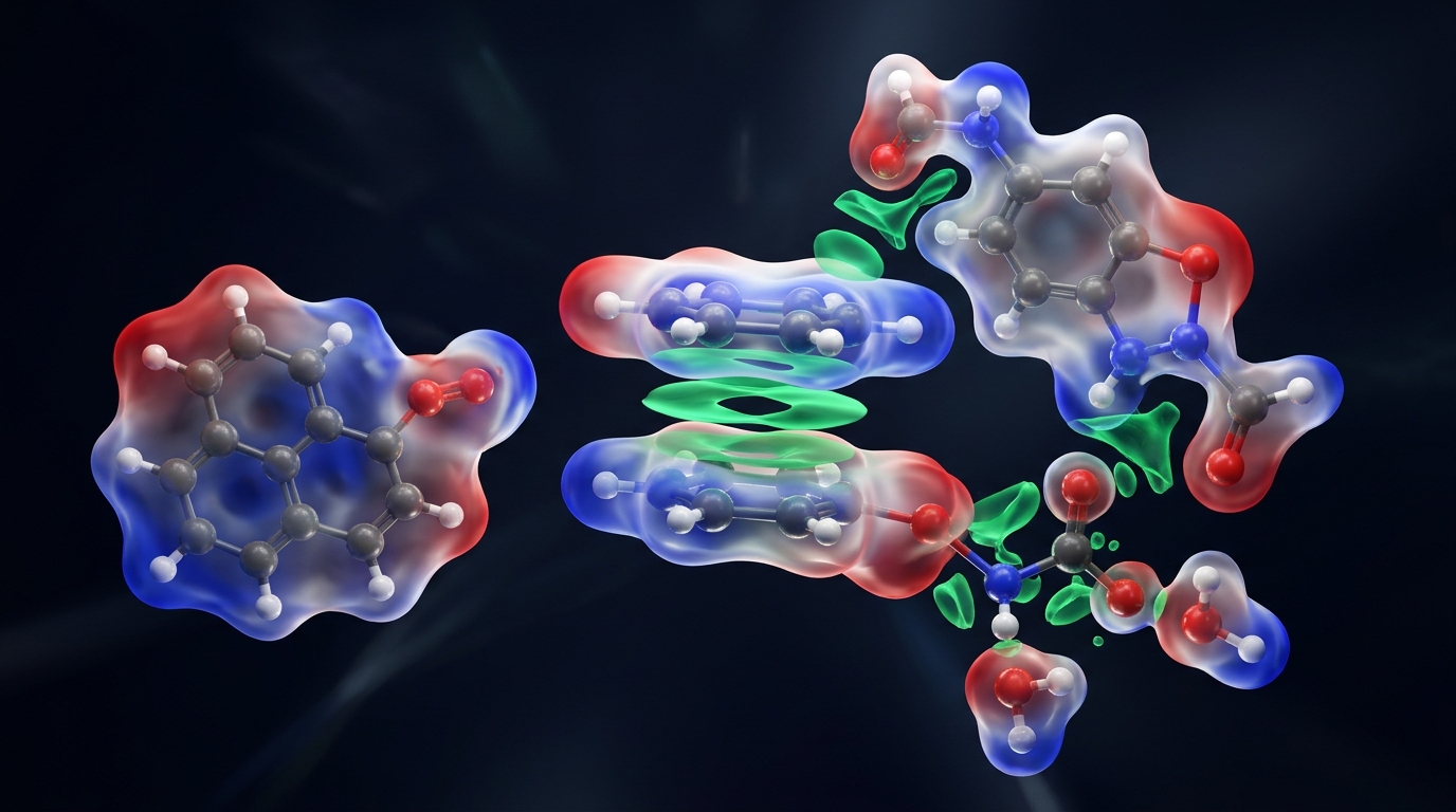
Ilustração 3D mostrando isosuperfícies de densidade eletrónica mapeadas com potencial eletrostático em vermelho e azul e discos verdes de interação não-covalente de dispersão pi-pi e ligações de hidrogénio

🌍 Ponto de Partida Químico e Ligação: Porque Precisamos Deste Capítulo?Chemical Starting Point & Connection: Why Do We Need This Chapter?

Bem-vindo ao Bloco IV! No Bloco III aprendemos a construir orbitais moleculares (LCAO-MO, Cap. 12) para sistemas muito simples como $\text{H}_2^+$ ou hidrocarbonetos $\pi$ de Hückel, onde os integrais eram tratados como parâmetros fixos ($\alpha, \beta$). Mas como é que um computador calcula, desde os primeiros princípios (ab initio, sem qualquer parâmetro experimental!), a geometria, o momento dipolar e as orbitais de uma molécula real como a aspirina, o colesterol ou um catalisador organometálico com $100$ eletrões? Welcome to Block IV! In Block III we learned how to build molecular orbitals (LCAO-MO, Ch. 12) for simple systems like $\text{H}_2^+$ or Hückel $\pi$ hydrocarbons, where integrals were treated as fixed parameters ($\alpha, \beta$). But how does a computer calculate, from first principles (ab initio, with zero experimental parameters!), the geometry, dipole moment, and orbitals of a real molecule like aspirin, cholesterol, or an organometallic catalyst with $100$ electrons?

O grande obstáculo, como vimos no Capítulo 9, é que a repulsão $\frac{1}{r_{12}}$ faz o movimento de cada eletrão depender instantaneamente da posição de todos os outros. A Teoria de Hartree–Fock (HF) resolve este impasse com uma ideia profundamente intuitiva: em vez de seguir cada colisão individual entre eletrões em tempo real, cada eletrão move-se independentemente dentro do "nevoeiro elétrico médio" (Campo Médio) criado pelos outros $N - 1$ eletrões! Neste capítulo vamos perceber como funciona o Ciclo de Campo Autoconsistente (SCF) que corre sempre que carrega em "Run" no ORCA ou no Gaussian, porque é que as energias das orbitais HOMO e LUMO têm significado experimental direto (Teorema de Koopmans), e porque é que o método RHF falha quando quebramos uma ligação covalente. The great obstacle, as we saw in Chapter 9, is that $\frac{1}{r_{12}}$ repulsion makes every electron's motion depend instantaneously on the position of every other electron. Hartree–Fock (HF) Theory breaks this deadlock with a deeply intuitive idea: instead of tracking every individual electron-electron collision in real time, each electron moves independently inside the "average electric fog" (Mean Field) created by the other $N - 1$ electrons! In this chapter we will understand how the Self-Consistent Field (SCF) Cycle works every time you hit "Run" in ORCA or Gaussian, why HOMO and LUMO orbital energies carry direct experimental meaning (Koopmans' Theorem), and why RHF breaks down when we stretch and break a covalent bond.

13.1 Aproximação de Campo Médio e os Operadores de Coulomb ($\hat{J}_j$), Troca ($\hat{K}_j$) e Fock ($\hat{f}$) 13.1 The Mean-Field Approximation and the Coulomb ($\hat{J}_j$), Exchange ($\hat{K}_j$), and Fock ($\hat{f}$) Operators

No Capítulo 10 vimos que a função de onda antissimétrica mais simples para $N$ eletrões é um único Determinante de Slater $\Phi_0 = |\chi_1 \chi_2 \cdots \chi_N\rangle$. A Teoria de Hartree–Fock (HF) junta o Capítulo 9 e o Capítulo 10 numa única pergunta: qual é o melhor Determinante de Slater único possível? Ou seja, aplicamos o Princípio Variacional para encontrar a forma das spin-orbitais ortonormais $\{\chi_i\}$ ($\langle \chi_i | \chi_j \rangle = \delta_{ij}$) que minimiza a energia total $E_{\text{HF}}[\{\chi_i\}] = \langle \Phi_0 | \hat{H}_{\text{el}} | \Phi_0 \rangle$. In Chapter 10 we saw that the simplest antisymmetric wavefunction for $N$ electrons is a single Slater Determinant $\Phi_0 = |\chi_1 \chi_2 \cdots \chi_N\rangle$. Hartree–Fock (HF) Theory combines Chapter 9 and Chapter 10 into one single question: what is the best possible single Slater Determinant? That is, we apply the Variational Principle to find the shapes of the orthonormal spin-orbitals $\{\chi_i\}$ ($\langle \chi_i | \chi_j \rangle = \delta_{ij}$) that minimize the total energy $E_{\text{HF}}[\{\chi_i\}] = \langle \Phi_0 | \hat{H}_{\text{el}} | \Phi_0 \rangle$.

💡 Analogia do Quotidiano — Conduzir Usando o Mapa do "Trânsito Médio Diário" (O Ciclo Autoconsistente SCF):Everyday Analogy — Driving Using the "Average Daily Traffic Map" (The Self-Consistent SCF Cycle): Como é que $N$ condutores numa cidade escolhem a melhor rota para o trabalho sem saberem a posição segundo a segundo de todos os outros carros? A aplicação GPS mostra o mapa médio de trânsito da cidade (a nuvem eletrónica média!). Cada condutor escolhe a sua rota ótima olhando para esse mapa médio. Mas claro: quando os condutores mudam de rota, o mapa de trânsito muda! Então a aplicação atualiza o mapa médio, os condutores voltam a ajustar as rotas, e o ciclo repete-se (10 a 20 iterações) até que o mapa de trânsito deixa de mudar — atingiu-se um Campo Autoconsistente (Self-Consistent Field, SCF)! How do $N$ commuters in a city choose their best route to work without knowing the second-by-second position of every other car? The GPS app displays the city's average traffic map (the average electron density cloud!). Each driver picks their optimal route based on that average map. Of course, once drivers change routes, the traffic map changes! So the app updates the average map, drivers adjust their routes again, and the cycle repeats (10 to 20 iterations) until the traffic map stops changing — reaching a Self-Consistent Field (SCF)!

Para uma molécula de camada fechada (Restricted Hartree–Fock, RHF) com $N$ eletrões emparelhados em $N/2$ orbitais espaciais $\{\phi_1, \dots, \phi_{N/2}\}$, a minimização variacional conduz às equações de Hartree–Fock, governadas pelo Operador de Fock efetivo de um eletrão $\hat{f}(1)$: For a closed-shell molecule (Restricted Hartree–Fock, RHF) with $N$ electrons paired in $N/2$ spatial orbitals $\{\phi_1, \dots, \phi_{N/2}\}$, variational minimization yields the Hartree–Fock equations governed by the effective one-electron Fock operator $\hat{f}(1)$:

EQUAÇÃO DE HARTREE–FOCK DE CAMADA FECHADA (RHF) E OPERADORES $\hat{J}_j$ E $\hat{K}_j$CLOSED-SHELL HARTREE–FOCK (RHF) EQUATION & OPERATORS $\hat{J}_j$ AND $\hat{K}_j$

$$\hat{f}(1)\phi_i(\mathbf{r}_1) = \varepsilon_i \phi_i(\mathbf{r}_1), \qquad \text{onde}\quad \hat{f}(1) = \hat{h}(1) + \sum_{j=1}^{N/2}\left[2\hat{J}_j(1) - \hat{K}_j(1)\right]$$ $$\begin{gathered} \hat{J}_j(1)\phi_i(\mathbf{r}_1) = \left[\int \frac{|\phi_j(\mathbf{r}_2)|^2}{r_{12}}\,d\mathbf{r}_2\right]\phi_i(\mathbf{r}_1) \quad (\text{Local}) \\[6pt] \hat{K}_j(1)\phi_i(\mathbf{r}_1) = \left[\int \frac{\phi_j^*(\mathbf{r}_2)\phi_i(\mathbf{r}_2)}{r_{12}}\,d\mathbf{r}_2\right]\phi_j(\mathbf{r}_1) \quad (\text{Não-Local!}) \end{gathered}$$

$$\hat{f}(1)\phi_i(\mathbf{r}_1) = \varepsilon_i \phi_i(\mathbf{r}_1), \qquad \text{where}\quad \hat{f}(1) = \hat{h}(1) + \sum_{j=1}^{N/2}\left[2\hat{J}_j(1) - \hat{K}_j(1)\right]$$ $$\begin{gathered} \hat{J}_j(1)\phi_i(\mathbf{r}_1) = \left[\int \frac{|\phi_j(\mathbf{r}_2)|^2}{r_{12}}\,d\mathbf{r}_2\right]\phi_i(\mathbf{r}_1) \quad (\text{Local}) \\[6pt] \hat{K}_j(1)\phi_i(\mathbf{r}_1) = \left[\int \frac{\phi_j^*(\mathbf{r}_2)\phi_i(\mathbf{r}_2)}{r_{12}}\,d\mathbf{r}_2\right]\phi_j(\mathbf{r}_1) \quad (\text{Nonlocal!}) \end{gathered}$$

🗣️ O que esta equação significa sem matemática:What this equation means without math: O operador de Fock $\hat{f}(1)$ é o "Hamiltoniano individual" sentido por um eletrão na molécula: inclui a sua energia cinética e atração pelos núcleos ($\hat{h}(1)$), mais a repulsão eletrostática média dos $2$ eletrões de cada orbital ocupada $j$ ($+2\hat{J}_j$), menos a correção quântica de troca de Pauli ($-\hat{K}_j$) com o eletrão de mesmo spin em cada orbital $j$. The Fock operator $\hat{f}(1)$ is the "effective one-electron Hamiltonian" felt by an electron in the molecule: it includes its kinetic energy and nuclear attraction ($\hat{h}(1)$), plus the average electrostatic repulsion from the $2$ electrons in each occupied orbital $j$ ($+2\hat{J}_j$), minus the quantum Pauli exchange correction ($-\hat{K}_j$) with the same-spin electron in each orbital $j$.

Repare na diferença estrutural entre $\hat{J}_j$ e $\hat{K}_j$: o Operador de Coulomb $\hat{J}_j(1)$ é um potencial multiplicativo local, ao passo que o Operador de Troca $\hat{K}_j(1)$ troca as etiquetas das orbitais $\phi_i \leftrightarrow \phi_j$ dentro do integral — é um operador integral não-local! E quando $i = j$, temos $\hat{J}_i(1)\phi_i(\mathbf{r}_1) = \hat{K}_i(1)\phi_i(\mathbf{r}_1)$, pelo que a troca de Hartree–Fock cancela exatamente a auto-repulsão espúria de Coulomb de cada eletrão consigo próprio ($\hat{J}_i - \hat{K}_i = 0$)! Notice the structural difference between $\hat{J}_j$ and $\hat{K}_j$: the Coulomb Operator $\hat{J}_j(1)$ is a local multiplicative potential, whereas the Exchange Operator $\hat{K}_j(1)$ swaps the orbital labels $\phi_i \leftrightarrow \phi_j$ inside the integral — it is a nonlocal integral operator! And when $i = j$, $\hat{J}_i(1)\phi_i(\mathbf{r}_1) = \hat{K}_i(1)\phi_i(\mathbf{r}_1)$, meaning that Hartree–Fock exchange cancels each electron's spurious self-Coulomb repulsion exactly ($\hat{J}_i - \hat{K}_i = 0$)!

13.2 Porque é que a Energia Total $E_{\text{HF}}$ NÃO é a Soma das Energias das Orbitais ($\sum_i \varepsilon_i$)? 13.2 Why Is the Total Energy $E_{\text{HF}}$ NOT the Sum of the Orbital Energies ($\sum_i \varepsilon_i$)?

Um erro muito comum entre estudantes que abrem pela primeira vez um ficheiro de output do ORCA ou do Gaussian é pensar que a energia eletrónica total da molécula é simplesmente a soma das energias das orbitais ocupadas ($\varepsilon_i$). A very common pitfall among students opening an ORCA or Gaussian output file for the first time is assuming that the total electronic energy of the molecule is simply the sum of the occupied orbital energies ($\varepsilon_i$).

Pense em dois vizinhos que partilham uma cerca que custou $100\text{ €}$ no total. Se perguntar ao Vizinho 1 "qual é o valor da cerca que tens ao pé da tua casa?", ele responde "$100\text{ €}$". Se perguntar ao Vizinho 2, ele também responde "$100\text{ €}$". Mas o custo total da cerca no bairro não é $100 + 100 = 200\text{ €}$ — é apenas $100\text{ €}$, porque a mesma cerca foi contada duas vezes! Think of two neighbors who share a fence that cost $100\text{ €}$ in total. If you ask Neighbor 1 "what is the value of the fence bordering your yard?", they answer "$100\text{ €}$". If you ask Neighbor 2, they also answer "$100\text{ €}$". Yet the total cost of the fence in the neighborhood is not $100 + 100 = 200\text{ €}$ — it is just $100\text{ €}$, because the exact same fence was counted twice!

💬 Questão Fundamental: «Se cada orbital ocupada tem energia $\varepsilon_i = \langle \phi_i | \hat{f} | \phi_i \rangle = h_{ii} + \sum_{j=1}^{N/2}(2J_{ij} - K_{ij})$, porque é que a energia eletrónica total de uma molécula RHF não é simplesmente $2\sum_{i=1}^{N/2}\varepsilon_i$?»Fundamental Question: "If each occupied orbital has energy $\varepsilon_i = \langle \phi_i | \hat{f} | \phi_i \rangle = h_{ii} + \sum_{j=1}^{N/2}(2J_{ij} - K_{ij})$, why isn't the total electronic energy of an RHF molecule simply $2\sum_{i=1}^{N/2}\varepsilon_i$?" Porque somar $\sum_i \varepsilon_i$ conta a repulsão entre cada par de eletrões DUAS VEZES! A energia da orbital $\varepsilon_1$ inclui a repulsão do eletrão $1$ com o eletrão $2$ ($J_{12}$), e a energia da orbital $\varepsilon_2$ inclui novamente a repulsão do eletrão $2$ com o eletrão $1$ ($J_{21} = J_{12}$). Para corrigir esta dupla contagem, temos de subtrair metade da interação intereletrónica total: Because summing $\sum_i \varepsilon_i$ counts the repulsion between every pair of electrons TWICE! The orbital energy $\varepsilon_1$ includes the repulsion of electron $1$ with electron $2$ ($J_{12}$), and the orbital energy $\varepsilon_2$ again includes the repulsion of electron $2$ with electron $1$ ($J_{21} = J_{12}$). To remove this double counting, we must subtract half of the total two-electron interaction: $$E_{\text{el}}^{\text{RHF}} = 2\sum_{i=1}^{N/2} h_{ii} + \sum_{i=1}^{N/2}\sum_{j=1}^{N/2}\left(2J_{ij} - K_{ij}\right) = 2\sum_{i=1}^{N/2} \varepsilon_i - \sum_{i=1}^{N/2}\sum_{j=1}^{N/2}\left(2J_{ij} - K_{ij}\right) = \sum_{i=1}^{N/2}\left(h_{ii} + \varepsilon_i\right)$$

13.3 As Equações Matriciais de Roothaan–Hall ($\mathbf{F}\mathbf{C} = \mathbf{S}\mathbf{C}\boldsymbol{\varepsilon}$), Ortogonalização $\mathbf{S}^{-1/2}$ e Ciclo SCF com DIIS 13.3 The Roothaan–Hall Matrix Equations ($\mathbf{F}\mathbf{C} = \mathbf{S}\mathbf{C}\boldsymbol{\varepsilon}$), $\mathbf{S}^{-1/2}$ Orthogonalization, and DIIS SCF Cycle

Em 1951, Clemens Roothaan e George Hall aplicaram a ideia de Rayleigh–Ritz (Cap. 9.3) às equações de Hartree–Fock: expandindo cada orbital molecular $\phi_i(\mathbf{r})$ num conjunto de $M$ funções de base atómicas conhecidas $\{\chi_\mu(\mathbf{r})\}_{\mu=1}^M$ ($\phi_i(\mathbf{r}) = \sum_{\nu=1}^M C_{\nu i}\chi_\nu(\mathbf{r})$), transformaram equações integro-diferenciais complicadas na equação matricial que corre em todos os computadores de química quântica do mundo: In 1951, Clemens Roothaan and George Hall applied the Rayleigh–Ritz idea (Ch. 9.3) to the Hartree–Fock equations: expanding each molecular orbital $\phi_i(\mathbf{r})$ in a basis of $M$ known atomic orbitals $\{\chi_\mu(\mathbf{r})\}_{\mu=1}^M$ ($\phi_i(\mathbf{r}) = \sum_{\nu=1}^M C_{\nu i}\chi_\nu(\mathbf{r})$), they transformed complicated integro-differential equations into the matrix equation that runs on every quantum chemistry computer in the world:

EQUAÇÕES DE ROOTHAAN–HALL, MATRIZ DENSIDADE $\mathbf{P}$ E ELEMENTOS DA MATRIZ DE FOCK $F_{\mu\nu}$ROOTHAAN–HALL EQUATIONS, DENSITY MATRIX $\mathbf{P}$ & FOCK MATRIX ELEMENTS $F_{\mu\nu}$ $$\begin{gathered} \mathbf{F}(\mathbf{P})\mathbf{C} = \mathbf{S}\mathbf{C}\boldsymbol{\varepsilon} \\[6pt] P_{\lambda\sigma} = 2\sum_{i=1}^{N/2} C_{\lambda i}C_{\sigma i}^* \\[6pt] F_{\mu\nu}(\mathbf{P}) = H_{\mu\nu}^{\text{core}} + \sum_{\lambda=1}^{M}\sum_{\sigma=1}^{M} P_{\lambda\sigma}\left[(\mu\nu|\lambda\sigma) - \frac{1}{2}(\mu\lambda|\sigma\nu)\right] \end{gathered}$$

🗣️ O que esta equação significa sem matemática:What this equation means without math: A matriz densidade $\mathbf{P}$ resume onde estão os eletrões na molécula. A partir de $\mathbf{P}$ e dos integrais de repulsão de dois eletrões $(\mu\nu|\lambda\sigma)$, o computador monta a matriz de Fock $\mathbf{F}(\mathbf{P})$ e diagonaliza-a (usando $\mathbf{S}^{-1/2}$) para encontrar novas orbitais $\mathbf{C}$ e energias $\boldsymbol{\varepsilon}$, repetindo o ciclo até que $\mathbf{P}$ deixe de mudar! The density matrix $\mathbf{P}$ summarizes where the electrons sit in the molecule. From $\mathbf{P}$ and the two-electron repulsion integrals $(\mu\nu|\lambda\sigma)$, the computer builds the Fock matrix $\mathbf{F}(\mathbf{P})$ and diagonalizes it (using $\mathbf{S}^{-1/2}$) to obtain updated orbitals $\mathbf{C}$ and energies $\boldsymbol{\varepsilon}$, repeating the loop until $\mathbf{P}$ stops changing!

Como a matriz de sobreposição atómica $\mathbf{S}$ não é a matriz identidade ($S_{\mu\nu} \neq \delta_{\mu\nu}$), o programa aplica a Ortogonalização Simétrica de Löwdin construindo $\mathbf{X} = \mathbf{S}^{-1/2}$: multiplicando à esquerda por $\mathbf{S}^{-1/2}$ e definindo $\mathbf{F}' = \mathbf{S}^{-1/2}\mathbf{F}\mathbf{S}^{-1/2}$ e $\mathbf{C}' = \mathbf{S}^{1/2}\mathbf{C}$, a equação reduz-se ao problema padrão de valores próprios $\mathbf{F}'\mathbf{C}' = \mathbf{C}'\boldsymbol{\varepsilon}$! Because the atomic overlap matrix $\mathbf{S}$ is not the identity matrix ($S_{\mu\nu} \neq \delta_{\mu\nu}$), the program applies Löwdin Symmetric Orthogonalization using $\mathbf{X} = \mathbf{S}^{-1/2}$: left-multiplying by $\mathbf{S}^{-1/2}$ and defining $\mathbf{F}' = \mathbf{S}^{-1/2}\mathbf{F}\mathbf{S}^{-1/2}$ and $\mathbf{C}' = \mathbf{S}^{1/2}\mathbf{C}$ transforms the generalized problem into the standard eigenvalue equation $\mathbf{F}'\mathbf{C}' = \mathbf{C}'\boldsymbol{\varepsilon}$!

🧪 Paralelo Real no Laboratório Computacional — O Erro SCF NOT CONVERGED e Como o Algoritmo DIIS de Pulay Salva o Seu Cálculo:Real-World Parallel in the Computational Lab — The SCF NOT CONVERGED Error & How Pulay's DIIS Algorithm Rescues Your Calculation: Todo o químico computacional já enfrentou o temido erro SCF NOT CONVERGED AFTER 125 CYCLES (especialmente em complexos de metais de transição com pequeno hiato HOMO–LUMO): na iteração 1 a carga salta para o ligante, na iteração 2 volta toda para o metal, oscilando indefinidamente (charge sloshing)! Para evitar isto, Péter Pulay inventou o algoritmo DIIS (Direct Inversion in the Iterative Subspace), que combina linearmente as matrizes de Fock das iterações anteriores para anular o vetor de erro $\mathbf{e}_k = \mathbf{F}_k\mathbf{P}_k\mathbf{S} - \mathbf{S}\mathbf{P}_k\mathbf{F}_k \to \mathbf{0}$ (e no ORCA moderno é complementado pelo otimizador de segunda ordem TRAH / SlowConv). Every computational chemist has faced the dreaded SCF NOT CONVERGED AFTER 125 CYCLES error (especially in transition-metal complexes with small HOMO–LUMO gaps): in iteration 1 charge sloshes onto the ligand, in iteration 2 it sloshes back onto the metal, oscillating endlessly! To cure this, Péter Pulay invented DIIS (Direct Inversion in the Iterative Subspace), which linearly combines Fock matrices from previous iterations to drive the commutator error $\mathbf{e}_k = \mathbf{F}_k\mathbf{P}_k\mathbf{S} - \mathbf{S}\mathbf{P}_k\mathbf{F}_k \to \mathbf{0}$ (and in modern ORCA is complemented by the second-order TRAH / SlowConv optimizer).

13.4 Teorema de Koopmans, Teorema de Brillouin e a Catástrofe de Dissociação RHF vs. UHF ($\langle \hat{S}^2 \rangle$) 13.4 Koopmans' Theorem, Brillouin's Theorem, and the RHF vs. UHF Dissociation Catastrophe ($\langle \hat{S}^2 \rangle$)

As orbitais e energias $\varepsilon_i$ que saem do ciclo SCF obedecem a dois teoremas fundamentais (Koopmans e Brillouin), mas escondem uma armadilha grave quando esticamos uma ligação covalente até a quebrar (a catástrofe RHF vs. UHF): The orbitals and energies $\varepsilon_i$ emerging from the SCF cycle obey two foundational theorems (Koopmans and Brillouin), yet hide a severe pitfall when we stretch a covalent bond to breaking (the RHF vs. UHF catastrophe):

Teorema de Koopmans (1934)Koopmans' Theorem (1934)

Potencial de Ionização Vertical ($\text{IP} \approx -\varepsilon_{\text{HOMO}}$):Vertical Ionization Potential ($\text{IP} \approx -\varepsilon_{\text{HOMO}}$):

$$\text{IP}_i = E_{\text{N}-1}^{\text{congelado}} - E_{\text{N}}^{\text{HF}} = -\varepsilon_i$$

$$\text{IP}_i = E_{\text{N}-1}^{\text{frozen}} - E_{\text{N}}^{\text{HF}} = -\varepsilon_i$$

Assumindo que as orbitais restantes não relaxam após remover 1 eletrão, $\text{IP}_{\text{vert}} \approx -\varepsilon_{\text{HOMO}}$ (os erros de ausência de relaxação orbital e de correlação eletrónica cancelam-se parcialmente nos potenciais de ionização!). Assuming the remaining orbitals stay frozen upon removing 1 electron, $\text{IP}_{\text{vert}} \approx -\varepsilon_{\text{HOMO}}$ (neglect of orbital relaxation and electron correlation partially cancel for ionization potentials!).

Teorema de Brillouin (1934)Brillouin's Theorem (1934)

Desacoplamento das Excitações Simples ($\Phi_i^a$):Zero Coupling to Singly Excited Determinants ($\Phi_i^a$):
$$\langle \Phi_0^{\text{HF}} | \hat{H}_{\text{el}} | \Phi_i^a \rangle = \langle \chi_i | \hat{f} | \chi_a \rangle = 0$$ Quando as orbitais convergem no ciclo SCF, a matriz de Fock é diagonal ($\langle i|\hat{f}|a\rangle = 0$). Por isso, as excitações simples $\Phi_i^a$ não se misturam diretamente com $\Phi_0$ na $1\text{ª}$ ordem da correlação! Once the SCF orbitals converge, the Fock matrix is diagonal ($\langle i|\hat{f}|a\rangle = 0$). Therefore, singly excited determinants $\Phi_i^a$ do not mix directly with $\Phi_0$ at first order!

Catástrofe RHF vs. UHFRHF vs. UHF Catastrophe

Dissociação Homolítica de $\text{H}_2$ e $\langle \hat{S}^2 \rangle$:Homolytic Dissociation of $\text{H}_2$ & $\langle \hat{S}^2 \rangle$:

$$\Phi_{\text{RHF}} \propto \underbrace{\left[\chi_A(1)\chi_B(2) + \chi_B(1)\chi_A(2)\right]}_{50\%\text{ Covalente }(\text{H}^\bullet + \text{H}^\bullet)} + \underbrace{\left[\chi_A(1)\chi_A(2) + \chi_B(1)\chi_B(2)\right]}_{50\%\text{ Iónico Espúrio }(\text{H}^+ + \text{H}^-)}$$

$$\Phi_{\text{RHF}} \propto \underbrace{\left[\chi_A(1)\chi_B(2) + \chi_B(1)\chi_A(2)\right]}_{50\%\text{ Covalent }(\text{H}^\bullet + \text{H}^\bullet)} + \underbrace{\left[\chi_A(1)\chi_A(2) + \chi_B(1)\chi_B(2)\right]}_{50\%\text{ Spurious Ionic }(\text{H}^+ + \text{H}^-)}$$

Em $R \to \infty$, o RHF inclui $50\%$ de termos iónicos $\text{H}^+\cdots\text{H}^-$, errando por $+7\text{ eV}$! O UHF permite que os eletrões $\alpha$ e $\beta$ se localizem em átomos opostos, recuperando a energia exata em $R \to \infty$, mas quebrando a simetria de spin ($\langle \hat{S}^2 \rangle \to 1.0$, mistura $50\%$ singleto + $50\%$ tripleto!). At $R \to \infty$, RHF retains $50\%$ ionic terms $\text{H}^+\cdots\text{H}^-$, overestimating energy by $+7\text{ eV}$! UHF lets $\alpha$ and $\beta$ electrons localize on opposite atoms, recovering the exact $R \to \infty$ energy at the cost of spin contamination ($\langle \hat{S}^2 \rangle \to 1.0$, $50\%$ singlet + $50\%$ triplet!).

💡 Analogia do Quotidiano — Dois Colegas de Casa Obrigados a Partilhar o Mesmo Quarto a $100\text{ km}$ de Distância (RHF vs. UHF):Everyday Analogy — Two Roommates Forced to Share the Same Bedroom $100\text{ km}$ Apart (RHF vs. UHF): No método RHF (Restricted Hartree–Fock), impomos que o eletrão $\uparrow$ e o eletrão $\downarrow$ partilhem exatamente a mesma orbital espacial $\sigma_g = \frac{1}{\sqrt{2(1+S)}}(\chi_A + \chi_B)$. Perto da distância de equilíbrio ($0.74\text{ Å}$), os dois átomos estão juntos na mesma casa e partilhar a sala é ótimo. Mas quando separamos os dois átomos de hidrogénio para $R = 100\text{ Å}$, obrigar os dois eletrões a continuar na orbital simétrica $\chi_A + \chi_B$ significa que 50% das vezes ambos os eletrões estão amontoados no mesmo átomo ($\text{H}^+ + \text{H}^-$)! O método UHF (Unrestricted Hartree–Fock) dá uma chave própria a cada eletrão: o eletrão $\uparrow$ vai morar para o átomo $A$ e o eletrão $\downarrow$ vai morar para o átomo $B$, dando a energia certa mas pagando o preço da contaminação de spin ($\langle \hat{S}^2 \rangle = 1.0$). In RHF (Restricted Hartree–Fock), we force the $\uparrow$ electron and the $\downarrow$ electron to share the exact same spatial orbital $\sigma_g = \frac{1}{\sqrt{2(1+S)}}(\chi_A + \chi_B)$. Near the equilibrium bond length ($0.74\text{ Å}$), both atoms live in the same house and sharing a room is fine. But when we pull the two hydrogen atoms apart to $R = 100\text{ Å}$, forcing both electrons to stay in the symmetric orbital $\chi_A + \chi_B$ means that 50% of the time both electrons are crammed onto the exact same atom ($\text{H}^+ + \text{H}^-$)! UHF (Unrestricted Hartree–Fock) gives each electron its own house key: the $\uparrow$ electron moves onto atom $A$ and the $\downarrow$ electron moves onto atom $B$, recovering the right dissociation energy at the price of spin contamination ($\langle \hat{S}^2 \rangle = 1.0$).

🧪 Paralelo Experimental — Espetroscopia Fotoeletrónica (UPS / XPS) e o Teorema de Koopmans:Experimental Parallel — Photoelectron Spectroscopy (UPS / XPS) & Koopmans' Theorem: Alguma vez lhe disseram que "orbitais não são observáveis"? Embora a função de onda em si não seja medida diretamente, na Espetroscopia Fotoeletrónica de Raios-X ou Ultravioleta (XPS / UPS) irradiamos uma molécula com fotões de energia conhecida $h\nu$ e medimos a energia cinética dos eletrões arrancados: cada pico do espetro experimental corresponde diretamente à energia de ionização de uma orbital ocupada, $\text{IP}_i \approx -\varepsilon_i$ (Teorema de Koopmans)! Por exemplo, no $\text{N}_2$ ou no $\text{H}_2\text{O}$, as posições dos picos fotoeletrónicos batem lado a lado com o diagrama das energias orbitais $\varepsilon_i$ de Hartree–Fock! Have you ever heard someone claim that "orbitals are not observables"? While a wavefunction itself is not measured directly, in Ultraviolet or X-ray Photoelectron Spectroscopy (UPS / XPS) we shine photons of known energy $h\nu$ on a molecule and measure the kinetic energy of the ejected electrons: each peak in the experimental spectrum maps directly onto the ionization energy of an occupied molecular orbital, $\text{IP}_i \approx -\varepsilon_i$ (Koopmans' Theorem)! For instance, in $\text{N}_2$ or $\text{H}_2\text{O}$, the photoelectron peaks line up one-for-one with the Hartree–Fock orbital energy diagram $\varepsilon_i$!

💬 Dúvida de Estudante: «Porque é que o Teorema de Koopmans funciona tão bem para potenciais de ionização ($\text{IP} \approx -\varepsilon_{\text{HOMO}}$), mas falha redondamente para afinidades eletrónicas ($\text{EA} \approx -\varepsilon_{\text{LUMO}}$)?»Student Question: "Why does Koopmans' Theorem work so well for ionization potentials ($\text{IP} \approx -\varepsilon_{\text{HOMO}}$), yet fail badly for electron affinities ($\text{EA} \approx -\varepsilon_{\text{LUMO}}$)?" Porque ao remover um eletrão (ionização), os dois erros que cometemos têm sinais opostos e cancelam-se: (1) ignorar a relaxação orbital torna o catião demasiado instável ($\text{IP}$ demasiado alto), enquanto (2) ignorar a correlação eletrónica (que é maior na molécula neutra com $N$ eletrões do que no catião com $N-1$ eletrões) torna o $\text{IP}$ demasiado baixo! Pelo contrário, ao adicionar um eletrão à LUMO para formar um anião ($N+1$ eletrões), a relaxação e a correlação somam-se na mesma direção, fazendo com que $\varepsilon_{\text{LUMO}}$ em Hartree–Fock seja quase sempre positivo (não ligado)! Because when removing an electron (ionization), the two errors we make have opposite signs and cancel: (1) neglecting orbital relaxation makes the cation too high in energy ($\text{IP}$ too large), whereas (2) neglecting electron correlation (which is larger in the $N$-electron neutral than in the $(N-1)$-electron cation) makes the $\text{IP}$ too small! Conversely, when adding an electron into the LUMO to form an $(N+1)$-electron anion, both relaxation and correlation errors add in the same direction, leaving the Hartree–Fock $\varepsilon_{\text{LUMO}}$ positive (unbound) in most molecules!

Exemplo Resolvido 13.1 — Cálculo Roothaan–Hall $\text{RHF/STO-3G}$ Completo para $\text{H}_2$ em $R = 1.40\,a_0$:Worked Example 13.1 — Complete Roothaan–Hall $\text{RHF/STO-3G}$ Calculation for $\text{H}_2$ at $R = 1.40\,a_0$:
Na base mínima $\text{STO-3G}$ em $R = 1.40\,a_0$ ($0.741\text{ Å}$), o integral de sobreposição vale $S_{12} = 0.6593$, os elementos de core valem $H_{11}^{\text{core}} = -1.1204\text{ E}_\text{h}$ e $H_{12}^{\text{core}} = -0.9584\text{ E}_\text{h}$, e a repulsão nuclear é $V_{NN} = \frac{1}{1.40} = +0.7143\text{ E}_\text{h}$. Por simetria molecular ($D_{\infty h}$), a orbital ocupada $\sigma_g$ tem coeficientes $C_{11} = C_{21} = \frac{1}{\sqrt{2(1 + S_{12})}} = 0.5489$, logo a matriz densidade converge imediatamente na $1\text{ª}$ iteração para $P_{11} = P_{12} = P_{22} = 2 C_{11}^2 = \frac{1}{1 + S_{12}} = \mathbf{0.6027}$. Construindo a matriz de Fock $\mathbf{F}(\mathbf{P})$, obtemos $\varepsilon_1(\sigma_g) = -0.5782\text{ E}_\text{h}$ (donde, pelo Teorema de Koopmans, $\text{IP}_{\text{vert}} \approx -\varepsilon_1 = +0.5782\text{ E}_\text{h} = 15.73\text{ eV}$, vs. experimental $15.43\text{ eV}$!), energia eletrónica $E_{\text{el}}^{\text{RHF}} = -1.8310\text{ E}_\text{h}$ e energia total $E_{\text{tot}}^{\text{RHF}} = E_{\text{el}}^{\text{RHF}} + V_{NN} = \mathbf{-1.1167\text{ E}_\text{h}}$. In the minimal $\text{STO-3G}$ basis at $R = 1.40\,a_0$ ($0.741\text{ Å}$), the overlap integral is $S_{12} = 0.6593$, the core elements are $H_{11}^{\text{core}} = -1.1204\text{ E}_\text{h}$ and $H_{12}^{\text{core}} = -0.9584\text{ E}_\text{h}$, and the nuclear repulsion is $V_{NN} = \frac{1}{1.40} = +0.7143\text{ E}_\text{h}$. By $D_{\infty h}$ symmetry, the occupied $\sigma_g$ orbital has coefficients $C_{11} = C_{21} = \frac{1}{\sqrt{2(1 + S_{12})}} = 0.5489$, so the density matrix converges immediately to $P_{11} = P_{12} = P_{22} = 2 C_{11}^2 = \frac{1}{1 + S_{12}} = \mathbf{0.6027}$. Forming $\mathbf{F}(\mathbf{P})$ gives $\varepsilon_1(\sigma_g) = -0.5782\text{ E}_\text{h}$ (so by Koopmans' theorem $\text{IP}_{\text{vert}} \approx -\varepsilon_1 = +0.5782\text{ E}_\text{h} = 15.73\text{ eV}$, vs. experimental $15.43\text{ eV}$!), electronic energy $E_{\text{el}}^{\text{RHF}} = -1.8310\text{ E}_\text{h}$, and total energy $E_{\text{tot}}^{\text{RHF}} = E_{\text{el}}^{\text{RHF}} + V_{NN} = \mathbf{-1.1167\text{ E}_\text{h}}$.

🔬 Interativo 13.1Interactive 13.1 Catástrofe de Dissociação RHF vs. Ponto de Coulson–Fischer UHF e Contaminação de Spin $\langle \hat{S}^2 \rangle$ em $\text{H}_2$ RHF Dissociation Catastrophe vs. UHF Coulson–Fischer Point & Spin Contamination $\langle \hat{S}^2 \rangle$ in $\text{H}_2$

🔬 Abrir Lab #14 / #16 →Open Lab #14 / #16 →

🎯 O Que Se Pretende Fazer Neste Simulador e Porquê What This Simulator Does & Why It Matters

Objetivo: Compreender o funcionamento do método de Hartree–Fock (SCF) e a sua falha clássica ao esticar uma ligação covalente (Capítulo 13): compare a curva RHF (que sobe para um limite errado por forçar termos iónicos $\text{H}^+\text{H}^-$) com a curva UHF (que quebra a simetria de spin) e a curva exata FCI. Goal: Understand how the Hartree–Fock (SCF) method works and why it fails when stretching a covalent bond (Chapter 13): compare the RHF curve (which rises to the wrong dissociation limit due to forced ionic $\text{H}^+\text{H}^-$ terms) against symmetry-broken UHF and exact FCI.

Distância Internuclear $R(\text{H–H})$ ($\text{ Å}$):Internuclear Distance $R(\text{H–H})$ ($\text{ Å}$): 0.74 Å (Equilíbrio)

ℹ️ Explicação deste seletor / controlo (clique para abrir)ℹ️ Explanation of this selector / control (click to open)

O que controla: Estica a ligação $R(\text{H–H})$ (em $\text{Å}$) desde o equilíbrio ($0.74\text{ Å}$) até à dissociação homolítica.
O que observar: Veja como o método restrito RHF falha ao dissociar (erro de correlação estática por forçar termos iónicos $\text{H}^+\text{H}^-$), enquanto UHF corrige a energia à custa de contaminação de spin ($\langle \hat{S}^2 \rangle \to 1.0$).What it controls: Stretches the $R(\text{H–H})$ bond (in $\text{Å}$) from equilibrium ($0.74\text{ Å}$) to homolytic dissociation.
What to observe: Watch how restricted RHF fails at dissociation (static correlation error from spurious ionic $\text{H}^+\text{H}^-$ terms), while UHF recovers the energy at the cost of spin contamination ($\langle \hat{S}^2 \rangle \to 1.0$).

Energia $\text{RHF}$$\text{RHF}$ Energy

-1.1336 Eh

Energia $\text{UHF}$$\text{UHF}$ Energy

-1.1336 Eh

Exata ($\text{FCI}$)Exact ($\text{FCI}$)

-1.1744 Eh

UHF $\langle \hat{S}^2 \rangle$ (Exato = $0$)UHF $\langle \hat{S}^2 \rangle$ (Exact = $0$)

0.000 (Puro Singleto)

📌 Mensagens-Chave para o Químico (Resumo sem Matemática) — Capítulo 13Key Takeaways for Chemists (Math-Free Summary) — Chapter 13

O que faz o Hartree–Fock (HF): Otimiza variacionalmente um único Determinante de Slater; cada eletrão move-se no campo eletrostático médio dos outros $N - 1$ eletrões ($\hat{J}_j$) mais a troca exata não-local de Pauli ($-\hat{K}_j$).What Hartree–Fock (HF) does: Variationally optimizes a single Slater Determinant; each electron moves in the average electrostatic field of the other $N - 1$ electrons ($\hat{J}_j$) plus exact nonlocal Pauli exchange ($-\hat{K}_j$).
Porque $E_{\text{HF}} \neq 2\sum_i \varepsilon_i$: Somar as energias das orbitais ocupadas conta a repulsão entre cada par de eletrões duas vezes; é preciso subtrair a repulsão intereletrónica total uma vez.Why $E_{\text{HF}} \neq 2\sum_i \varepsilon_i$: Summing occupied orbital energies double-counts every electron-pair repulsion; the total two-electron repulsion must be subtracted once.
Equações de Roothaan–Hall ($\mathbf{F}\mathbf{C} = \mathbf{S}\mathbf{C}\boldsymbol{\varepsilon}$) e Teorema de Koopmans: Expandir as MOs numa base atómica transforma o HF num ciclo matricial autoconsistente (SCF), onde $-\varepsilon_{\text{HOMO}}$ estima a energia de ionização vertical.Roothaan–Hall Equations ($\mathbf{F}\mathbf{C} = \mathbf{S}\mathbf{C}\boldsymbol{\varepsilon}$) and Koopmans' Theorem: Expanding MOs in an atomic basis turns HF into a self-consistent matrix cycle (SCF), where $-\varepsilon_{\text{HOMO}}$ estimates the vertical ionization potential.
RHF vs. UHF na quebra homolítica de ligações: O RHF falha ao quebrar uma ligação covalente porque impõe $50\%$ de caráter iónico espúrio ($\text{H}^+\text{H}^-$); o UHF corrige a energia separando os spins $\alpha$ e $\beta$ em átomos opostos, mas introduz contaminação de spin ($\langle \hat{S}^2 \rangle > 0$).RHF vs. UHF in homolytic bond breaking: RHF fails when breaking a covalent bond because it enforces $50\%$ spurious ionic character ($\text{H}^+\text{H}^-$); UHF fixes the dissociation energy by localizing $\alpha$ and $\beta$ spins on opposite atoms, at the cost of spin contamination ($\langle \hat{S}^2 \rangle > 0$).

🎯 Questionário de Conceitos Fundamentais — Capítulo 13 — Teoria de Campo Autoconsistente de Hartree–Fock (SCF), Equações de Roothaan–Hall ($\mathbf{F}\mathbf{C} = \mathbf{S}\mathbf{C}\boldsymbol{\varepsilon}$), RHF vs. UHF e Teorema de KoopmansCore Concepts Questionnaire — Chapter 13 — Hartree–Fock Self-Consistent Field Theory (SCF), Roothaan–Hall Equations ($\mathbf{F}\mathbf{C} = \mathbf{S}\mathbf{C}\boldsymbol{\varepsilon}$), RHF vs. UHF, and Koopmans' Theorem

Questões acessíveis sobre os conceitos essenciais deste capítulo • Clique em «Outra Variante» ou «Feedback de Estudo» para saber o que estudar mais.Accessible questions on this chapter's essential concepts • Click "Swap Variant" or "Study Feedback" for personalized study guidance.

0 / 4 (0%)

🔗 Texto de Ligação para o Próximo CapítuloBridge to the Next Chapter

Nas Equações de Roothaan–Hall ($\mathbf{F}\mathbf{C} = \mathbf{S}\mathbf{C}\boldsymbol{\varepsilon}$), toda a qualidade da função de onda molecular depende das $M$ funções de base atómicas $\{\chi_\mu(\mathbf{r})\}$ que escolhemos para construir as colunas de $\mathbf{C}$. Quando abre um ficheiro de input do ORCA ou do Gaussian, vê siglas misteriosas ao lado do método — como STO-3G, 6-31G*, cc-pVTZ ou def2-TZVPP. O que significam exatamente essas letras e números? Porque é que escolher a base errada pode arruinar completamente um cálculo sobre um anião ou sobre uma ponte de hidrogénio? No Capítulo 14, vamos aprender a escolher e dominar os Conjuntos de Base Atómicos! In the Roothaan–Hall Equations ($\mathbf{F}\mathbf{C} = \mathbf{S}\mathbf{C}\boldsymbol{\varepsilon}$), the entire quality of the molecular wavefunction hinges on the $M$ atomic basis functions $\{\chi_\mu(\mathbf{r})\}$ we choose to build the columns of $\mathbf{C}$. Whenever you open an ORCA or Gaussian input file, you see mysterious acronyms next to the method — such as STO-3G, 6-31G*, cc-pVTZ, or def2-TZVPP. What do those letters and numbers actually mean? Why can picking the wrong basis set completely ruin a calculation on an anion or a hydrogen bond? In Chapter 14, we will learn how to choose and master Atomic Basis Sets!

14

Capítulo 14 — Conjuntos de Base Atómicos: Orbitais de Slater (STO) vs. Gaussianas (GTO), Bases Pople, Dunning ($\text{cc-pVXZ}$), Karlsruhe ($\text{def2-TZVP}$), Extrapolação CBS e BSSE Chapter 14 — Atomic Basis Sets: Slater (STO) vs. Gaussian (GTO) Orbitals, Pople, Dunning ($\text{cc-pVXZ}$), Karlsruhe ($\text{def2-TZVP}$), CBS Extrapolation, and BSSE

Como escolher e auditar o conjunto de funções matemáticas $\{\chi_\mu(\mathbf{r})\}$ usado para representar as orbitais moleculares num computador. How to choose and audit the mathematical basis set $\{\chi_\mu(\mathbf{r})\}$ used to represent molecular orbitals on a computer.

🌍 Ponto de Partida Químico e Ligação: Porque Precisamos Deste Capítulo?Chemical Starting Point & Connection: Why Do We Need This Chapter?

No Capítulo 13 aprendemos o truque que tornou a Química Computacional possível: a expansão $\text{LCAO-MO}$ de Roothaan–Hall transforma as equações integro-diferenciais de Hartree–Fock num problema de matrizes resolúvel por computador, expandindo cada orbital molecular como uma soma linear de funções matemáticas pré-escolhidas centradas nos átomos. Mas deixámos em aberto a pergunta prática mais decisiva de todas: quais são exatamente essas funções de base atómicas? In Chapter 13 we learned the breakthrough that made Computational Chemistry possible: the Roothaan–Hall $\text{LCAO-MO}$ expansion turns the coupled Hartree–Fock integro-differential equations into a computer-solvable matrix problem by expanding each molecular orbital as a linear combination of pre-selected mathematical basis functions centered on the atoms. Yet we left the most decisive practical question wide open: what exactly are those atomic basis functions?

Sempre que escreve a primeira linha de um ficheiro de input para o ORCA, Gaussian ou Q-Chem — por exemplo, ! B3LYP def2-TZVP ou ! CCSD(T) aug-cc-pVTZ — a segunda sigla é o conjunto de base atómico (basis set). Escolher um conjunto de base inadequado é o erro mais frequente e mais silencioso da Química Computacional: se tentar calcular a afinidade eletrónica do cloro ($\text{Cl} + e^- \to \text{Cl}^-$) sem funções difusas, ou a geometria do dióxido de enxofre ($\text{SO}_2$) sem funções de polarização $d$, mesmo o método quântico mais caro do mundo devolverá resultados qualitativamente errados! Whenever you type the first line of an input file for ORCA, Gaussian, or Q-Chem — such as ! B3LYP def2-TZVP or ! CCSD(T) aug-cc-pVTZ — the second keyword is the atomic basis set. Choosing an inadequate basis set is the single most common and silent error in Computational Chemistry: if you try to compute the electron affinity of chlorine ($\text{Cl} + e^- \to \text{Cl}^-$) without diffuse functions, or the geometry of sulfur dioxide ($\text{SO}_2$) without $d$ polarization functions, even the most expensive quantum method in the world will return qualitatively wrong answers!

Neste capítulo vamos desmistificar todo o «alfabeto sopa de letras» das bases modernas ($\text{STO-3G}$, $6\text{-}31\text{G(d,p)}$, $\text{cc-pVTZ}$, $\text{def2-TZVP}$, $\text{ma-def2-TZVP}$). Vai compreender porque trocamos funções exponenciais exatas de Slater por Gaussianas de Boys, quando é obrigatório adicionar funções de polarização ou difusas, como funcionam os pseudopotenciais relativísticos ($\text{ECPs}$) em metais pesados como o Ouro e a Platina, e como eliminar o erro de sobreposição do conjunto de base ($\text{BSSE}$) em ligações de hidrogénio e interações fármaco-recetor. In this chapter we will demystify the entire "alphabet soup" of modern basis sets ($\text{STO-3G}$, $6\text{-}31\text{G(d,p)}$, $\text{cc-pVTZ}$, $\text{def2-TZVP}$, $\text{ma-def2-TZVP}$). You will understand why we trade exact exponential Slater functions for Boys Gaussians, when polarization and diffuse functions are mandatory, how relativistic Effective Core Potentials ($\text{ECPs}$) work in heavy metals like Gold and Platinum, and how to eliminate Basis Set Superposition Error ($\text{BSSE}$) in hydrogen bonds and drug–receptor interactions.

14.1 Orbitais de Slater (STO, $e^{-\zeta r}$) vs. Gaussianas (GTO, $e^{-\alpha r^2}$) e o Teorema do Produto Gaussiano de Boys (1950) 14.1 Slater (STO, $e^{-\zeta r}$) vs. Gaussian (GTO, $e^{-\alpha r^2}$) Orbitals and Boys' Gaussian Product Theorem (1950)

As soluções analíticas exatas de átomos hidrogenoides têm decaimento radial exponencial, chamado Orbitais do Tipo Slater (STO — Slater-Type Orbitals), $\chi^{\text{STO}}(\mathbf{r}) \propto r^{n-1}e^{-\zeta r}Y_{lm}(\theta,\phi)$. As STOs possuem duas propriedades físicas exatas: (1) uma cúspide nuclear aguda de Kato em $r \to 0$ ($\left.\frac{d\chi}{dr}\right|_{r=0} = -\zeta\chi(0) \neq 0$), e (2) um decaimento exponencial correto a longa distância ($e^{-\zeta r}$). Então, porque é que quase nenhum programa molecular poliatómico usa STOs? Exact analytical solutions of hydrogenic atoms have exponential radial decay, called Slater-Type Orbitals (STOs), $\chi^{\text{STO}}(\mathbf{r}) \propto r^{n-1}e^{-\zeta r}Y_{lm}(\theta,\phi)$. STOs possess two exact physical properties: (1) a sharp Kato nuclear cusp at $r \to 0$ ($\left.\frac{d\chi}{dr}\right|_{r=0} = -\zeta\chi(0) \neq 0$), and (2) the correct long-range exponential tail ($e^{-\zeta r}$). Why, then, do almost no polyatomic molecular programs use STOs?

Porque num cálculo molecular precisamos de calcular milhões a biliões de integrais de repulsão de dois eletrões centrados em quatro átomos diferentes $(\mu_A\nu_B|\lambda_C\sigma_D)$, que não têm fórmula analítica fechada para STOs! Em 1950, S. Francis Boys revolucionou a Química Computacional ao substituir $e^{-\zeta r}$ por Orbitais do Tipo Gaussiano (GTO — Gaussian-Type Orbitals), $g(\alpha, \mathbf{r}-\mathbf{R}_A) \propto (x-X_A)^{l_x}(y-Y_A)^{l_y}(z-Z_A)^{l_z}e^{-\alpha|\mathbf{r}-\mathbf{R}_A|^2}$, graças ao Teorema do Produto Gaussiano: Because in a molecular calculation we must evaluate millions to billions of two-electron repulsion integrals centered on four different atoms $(\mu_A\nu_B|\lambda_C\sigma_D)$, which have no closed analytical formula for STOs! In 1950, S. Francis Boys revolutionized Computational Chemistry by replacing $e^{-\zeta r}$ with Gaussian-Type Orbitals (GTOs), $g(\alpha, \mathbf{r}-\mathbf{R}_A) \propto (x-X_A)^{l_x}(y-Y_A)^{l_y}(z-Z_A)^{l_z}e^{-\alpha|\mathbf{r}-\mathbf{R}_A|^2}$, thanks to the Gaussian Product Theorem:

TEOREMA DO PRODUTO GAUSSIANO DE BOYS (1950) E CONTRAÇÃO $\text{CGTO}$BOYS' GAUSSIAN PRODUCT THEOREM (1950) & $\text{CGTO}$ CONTRACTION

$$\begin{gathered} e^{-\alpha |\mathbf{r} - \mathbf{R}_A|^2} \times e^{-\beta |\mathbf{r} - \mathbf{R}_B|^2} = K_{AB}\,e^{-p |\mathbf{r} - \mathbf{R}_P|^2} \\[6pt] \text{onde } p = \alpha + \beta, \quad \mathbf{R}_P = \frac{\alpha\mathbf{R}_A + \beta\mathbf{R}_B}{\alpha + \beta}, \quad K_{AB} = \exp\!\left(-\frac{\alpha\beta}{\alpha+\beta}|\mathbf{R}_A - \mathbf{R}_B|^2\right) \end{gathered}$$ $$\begin{gathered} \chi_\mu^{\text{CGTO}}(\mathbf{r} - \mathbf{R}_A) = \sum_{p=1}^{L} d_{p\mu}\,g_p(\alpha_{p\mu}, \mathbf{r} - \mathbf{R}_A) \\[6pt] (\text{Combinação fixa de }L\text{ primitivas Gaussianas}) \end{gathered}$$

$$\begin{gathered} e^{-\alpha |\mathbf{r} - \mathbf{R}_A|^2} \times e^{-\beta |\mathbf{r} - \mathbf{R}_B|^2} = K_{AB}\,e^{-p |\mathbf{r} - \mathbf{R}_P|^2} \\[6pt] \text{where } p = \alpha + \beta, \quad \mathbf{R}_P = \frac{\alpha\mathbf{R}_A + \beta\mathbf{R}_B}{\alpha + \beta}, \quad K_{AB} = \exp\!\left(-\frac{\alpha\beta}{\alpha+\beta}|\mathbf{R}_A - \mathbf{R}_B|^2\right) \end{gathered}$$ $$\begin{gathered} \chi_\mu^{\text{CGTO}}(\mathbf{r} - \mathbf{R}_A) = \sum_{p=1}^{L} d_{p\mu}\,g_p(\alpha_{p\mu}, \mathbf{r} - \mathbf{R}_A) \\[6pt] (\text{Fixed linear combination of }L\text{ primitive Gaussians}) \end{gathered}$$

🗣️ Tradução em linguagem corrente: A primeira equação é um autêntico milagre algébrico: quando multiplicamos duas funções Gaussianas centradas em átomos diferentes ($\mathbf{R}_A$ e $\mathbf{R}_B$), o resultado é uma única Gaussiana centrada num ponto intermédio $\mathbf{R}_P$ sobre a linha que une os dois átomos! Isto transforma um integral impossível de 4 centros num integral simples de 2 centros que um computador calcula em nanossegundos. A segunda equação mostra como corrigimos a forma redonda das Gaussianas: somamos $L$ Gaussianas primitivas (umas estreitas junto ao núcleo, outras largas na cauda) com pesos fixos $d_{p\mu}$ para imitar fielmente uma orbital física de Slater. 🗣️ Plain-English translation: The first equation is an algebraic miracle: when you multiply two Gaussian functions centered on different atoms ($\mathbf{R}_A$ and $\mathbf{R}_B$), the product is a single Gaussian centered at an intermediate point $\mathbf{R}_P$ along the line connecting the two atoms! This turns an intractable 4-center integral into a simple 2-center integral that a computer evaluates in nanoseconds. The second equation shows how we fix the rounded shape of Gaussians: we sum $L$ primitive Gaussians (some tight near the nucleus, others broad in the tail) with fixed weights $d_{p\mu}$ to faithfully mimic a physical Slater orbital.

O produto de duas Gaussianas centradas em átomos diferentes $A$ e $B$ é uma única Gaussiana centrada num ponto intermédio $\mathbf{R}_P$ do segmento $AB$! Assim, todo o integral de 4 centros reduz-se imediatamente a um integral analítico ultrarrápido de 2 centros. Para compensar o facto de uma única Gaussiana ter derivada nula no núcleo ($\left.\frac{d}{dr}e^{-\alpha r^2}\right|_{r=0} = 0$, sem cúspide!) e decair demasiado depressa a longa distância ($e^{-\alpha r^2}$), combinamos $L$ Gaussianas primitivas (com expoentes $\alpha_p$ grandes para o núcleo e pequenos para a cauda) numa Gaussiana Contraída ($\text{CGTO}$) com coeficientes fixos $d_{p\mu}$ (por exemplo, na base mínima histórica $\text{STO-3G}$, ajustam-se $L=3$ Gaussianas a cada STO). The product of two Gaussians centered on different atoms $A$ and $B$ is a single Gaussian centered at an intermediate point $\mathbf{R}_P$ along the line segment $AB$! Consequently, every 4-center integral reduces immediately to an ultra-fast analytical 2-center integral. To compensate for a single Gaussian having zero slope at the nucleus ($\left.\frac{d}{dr}e^{-\alpha r^2}\right|_{r=0} = 0$, no cusp!) and decaying too rapidly at long range ($e^{-\alpha r^2}$), we combine $L$ primitive Gaussians (with tight exponents $\alpha_p$ near the nucleus and diffuse exponents in the tail) into a Contracted Gaussian ($\text{CGTO}$) with fixed coefficients $d_{p\mu}$ (for example, in the historical minimal basis $\text{STO-3G}$, $L=3$ primitives are fitted to each STO).

💡 Analogia — Esculpir uma Esfera com Blocos de LEGO (STO-3G vs. def2-TZVP): Imagine que quer construir uma escultura perfeitamente curva da nuvem eletrónica de uma molécula usando peças de LEGO. Uma Orbital de Slater ($\text{STO}$) seria uma peça de cerâmica moldada à medida — perfeita para um átomo isolado, mas impossível de encaixar rapidamente com outras. As Gaussianas ($\text{GTO}$) são blocos de LEGO padronizados que encaixam instantaneamente uns nos outros (Teorema do Produto Gaussiano). Usar uma base mínima como STO-3G é como tentar esculpir um rosto humano usando apenas 3 tijolos DUPLO gigantes por átomo: fica quadrado, rígido e irreconhecível. Usar uma base moderna como def2-TZVP ou cc-pVQZ é como dispor de centenas de peças LEGO de todos os tamanhos e inclinações, permitindo reproduzir cada curva subtil da densidade eletrónica! 💡 Analogy — Sculpting a Sphere with LEGO Bricks (STO-3G vs. def2-TZVP): Imagine trying to build a smoothly curved sculpture of a molecule's electron cloud using LEGO bricks. A Slater-Type Orbital ($\text{STO}$) is like a custom-molded ceramic piece — exact for a single atom, but nearly impossible to interlock rapidly with neighboring pieces. Gaussian-Type Orbitals ($\text{GTOs}$) are standardized LEGO bricks that snap together instantaneously (Boys' Gaussian Product Theorem). Using a minimal basis set like STO-3G is like trying to sculpt a human face using only 3 giant square DUPLO blocks per atom: blocky, rigid, and unrecognizable. Using a modern basis set like def2-TZVP or cc-pVQZ gives you hundreds of fine LEGO bricks of different sizes and angles, allowing you to capture every subtle contour of the electron density!

14.2 Valência Dividida (Double/Triple/Quadruple-Zeta), Funções de Polarização e Funções Difusas 14.2 Split-Valence (Double/Triple/Quadruple-Zeta), Polarization Functions, and Diffuse Functions

Quando um átomo deixa de estar isolado no vácuo e passa a fazer parte de uma molécula, a sua nuvem eletrónica sofre três tipos de deformações físicas fundamentais: (1) contrai-se ou expande-se radialmente conforme a eletronegatividade dos vizinhos; (2) deforma-se angularmente na direção das ligações químicas; e (3) em aniões ou estados fracamente ligados, espalha-se até grandes distâncias do núcleo. When an atom is no longer isolated in vacuum and becomes part of a molecule, its electron cloud undergoes three fundamental physical deformations: (1) it contracts or expands radially depending on the electronegativity of its neighbors; (2) it distorts angularly toward the chemical bonds; and (3) in anions or weakly bound states, it spreads out far from the nucleus.

Como as funções de base individuais têm expoentes fixos $\alpha$, a única forma de dar liberdade à nuvem eletrónica para realizar estas três adaptações é fornecer três ingredientes matemáticos específicos no conjunto de base: valência dividida ($n\text{-}\zeta$), funções de polarização e funções difusas. Because individual basis functions have fixed exponents $\alpha$, the only way to give the electron cloud the freedom to perform these three adaptations is to supply three specific mathematical ingredients in the basis set: split valence ($n\text{-}\zeta$), polarization functions, and diffuse functions.

1. Valência Dividida ($n\text{-}\zeta$)1. Split Valence ($n\text{-}\zeta$)

Flexibilidade Radial ($\text{DZ}, \text{TZ}, \text{QZ}$):Radial Flexibility ($\text{DZ}, \text{TZ}, \text{QZ}$):
Durante a formação de uma ligação química, as orbitais de valência precisam de contrair ou expandir radialmente. Uma base Dupla-Zeta (DZ) fornece 2 funções de tamanhos diferentes por orbital de valência; Tripla-Zeta (TZ) fornece 3; Quádrupla-Zeta (QZ) fornece 4. During bond formation, valence orbitals must contract or expand radially. A Double-Zeta (DZ) basis provides 2 functions of different radial sizes per valence orbital; Triple-Zeta (TZ) provides 3; Quadruple-Zeta (QZ) provides 4.

2. Funções de Polarização ($l + 1$)2. Polarization Functions ($l + 1$)

Flexibilidade Angular ($d, f$ em C/N/O; $p$ em H):Angular Flexibility ($d, f$ on C/N/O; $p$ on H):
Adicionar funções de momento angular superior ($p$ no Hidrogénio; $d$ e $f$ no Carbono, Azoto, Oxigénio) permite que a nuvem eletrónica se desloque para fora do átomo e se concentre na região internuclear da ligação (essencial para geometrias piramidais como $\text{NH}_3$ e hipervalentes como $\text{SO}_2$). Adding higher angular momentum functions ($p$ on Hydrogen; $d$ and $f$ on Carbon, Nitrogen, Oxygen) allows the electron cloud to shift toward the internuclear bonding region (mandatory for pyramidal $\text{NH}_3$ and hypervalent $\text{SO}_2$).

3. Funções Difusas (+, aug-, ma-)3. Diffuse Functions (+, aug-, ma-)

Caudas Espaciais Longas ($\alpha$ pequeno):Long Spatial Tails (Small $\alpha$):
Gaussianas com expoentes $\alpha \ll 0.1\,a_0^{-2}$ que se estendem longe dos núcleos. São obrigatórias em aniões ($\text{F}^-, \text{OH}^-$), afinidades eletrónicas, estados excitados de Rydberg e interações não-covalentes fracas! Gaussians with very small exponents $\alpha \ll 0.1\,a_0^{-2}$ extending far from the nuclei. They are mandatory for anions ($\text{F}^-, \text{OH}^-$), electron affinities, Rydberg excited states, and weak noncovalent interactions!

🧪 Química no Mundo Real — Porque é que os Aniões ($\text{F}^-$, $\text{OH}^-$) e o $\text{NH}_3$ Colapsam sem as Funções Certas?Real-World Chemistry — Why Do Anions ($\text{F}^-$, $\text{OH}^-$) and $\text{NH}_3$ Fail Without the Right Functions? Dois exemplos clássicos de laboratório demonstram porque não podemos poupar nas funções de polarização e difusas: (1) Se otimizar a geometria do amoníaco ($\text{NH}_3$) sem funções de polarização $d$ no azoto, a molécula fica completamente plana (trigonal planar, $D_{3h}$) em vez de piramidal, porque as orbitais $2p$ rígidas não conseguem inclinar o par isolado! (2) Se calcular a reação de formação do ião fluoreto $\text{F(g)} + e^- \to \text{F}^-\text{(g)}$ com a base cc-pVDZ (sem funções difusas), o computador prevê que o ião $\text{F}^-$ é instável face à perda do eletrão! Porquê? Porque o eletrão extra num anião está fracamente ligado e habita uma nuvem muito larga; sem funções difusas (aug-cc-pVDZ ou ma-def2-TZVP), o eletrão é artificialmente comprimido contra os outros 9 eletrões do flúor, disparando a repulsão de Coulomb! Two classic laboratory examples show why we cannot skimp on polarization and diffuse functions: (1) If you optimize the geometry of ammonia ($\text{NH}_3$) without $d$ polarization functions on nitrogen, the molecule comes out completely flat (trigonal planar, $D_{3h}$) instead of pyramidal, because rigid $2p$ orbitals cannot bend the lone pair! (2) If you compute the electron affinity of fluorine $\text{F(g)} + e^- \to \text{F}^-\text{(g)}$ with cc-pVDZ (no diffuse functions), the computer predicts that $\text{F}^-$ is unstable with respect to losing the electron! Why? Because the extra electron in an anion is loosely bound and occupies a very broad cloud; without diffuse functions (aug-cc-pVDZ or ma-def2-TZVP), that electron is artificially squeezed against fluorine's other 9 electrons, causing Coulomb repulsion to skyrocket!

💬 Dúvida de Aluno: «O átomo de Hidrogénio só tem 1 eletrão na orbital $1s$. Porque é que uma base como 6-31G(d,p) ou def2-TZVP coloca orbitais $p$ e $d$ no Hidrogénio?! O eletrão vai ser promovido para $2p$?»Student Question: "The Hydrogen atom only has 1 electron in the $1s$ orbital. Why does a basis set like 6-31G(d,p) or def2-TZVP put $p$ and $d$ orbitals on Hydrogen?! Is the electron being promoted to $2p$?" Não! Na Química Computacional chamamos-lhes funções de polarização, e não orbitais excitadas. Uma orbital $1s$ pura é perfeitamente esférica em torno do protão. Mas quando o átomo de Hidrogénio se liga a um átomo de Flúor em $\text{HF}$, a nuvem eletrónica do Hidrogénio é puxada para o lado do Flúor — deixa de ser esférica! Matematicamente, a única maneira de deslocar o centro de uma esfera $s$ ligeiramente para a direita é somar-lhe uma pequena fração de uma função $p_z$ (que tem sinal positivo à direita e negativo à esquerda). Portanto, as funções $p$ no Hidrogénio (e $d$ no Carbono) servem como «ferramentas de moldagem angular» para deformar a nuvem eletrónica na direção das ligações químicas! No! In Computational Chemistry we call them polarization functions, not excited orbitals. A pure $1s$ orbital is perfectly spherical around the proton. But when a Hydrogen atom bonds to Fluorine in $\text{HF}$, Hydrogen's electron cloud is pulled toward Fluorine — it is no longer centered on the proton! Mathematically, the only way to shift the center of a spherical $s$ function slightly to the right is to mix in a small fraction of a $p_z$ function (which has a positive lobe on the right and a negative lobe on the left). Thus, $p$ functions on Hydrogen (and $d$ functions on Carbon) act as "angular shaping tools" to deform the electron cloud toward chemical bonds!

14.3 As 3 Famílias de Conjuntos de Base Modernos e Potenciais Efetivos de Core (ECPs) 14.3 The 3 Modern Basis Set Families and Effective Core Potentials (ECPs)

Ao longo das últimas cinco décadas, dezenas de conjuntos de base foram propostos, mas na prática moderna quase todos os cálculos em Química Orgânica, Inorgânica e Bioquímica utilizam uma de três grandes famílias sistemáticas: as bases de Karlsruhe (Ahlrichs/Weigend, família def2), as bases consistentes na correlação de Dunning (família cc-pVXZ) e as bases históricas de valência dividida de Pople (família 6-31G). Over the past five decades, dozens of basis sets have been proposed, yet in modern practice almost all calculations in Organic, Inorganic, and Biological Chemistry rely on one of three systematic families: the Karlsruhe basis sets (Ahlrichs/Weigend, def2 family), Dunning's correlation-consistent basis sets (cc-pVXZ family), and Pople's historical split-valence basis sets (6-31G family).

Cada família foi desenhada com um objetivo específico em mente: as bases def2 de Karlsruhe são otimizadas para convergir rapidamente em cálculos de Teoria do Funcional da Densidade (DFT) em toda a Tabela Periódica (do Hidrogénio ao Rádon); já as bases cc-pVXZ de Thom Dunning foram desenhadas especificamente para recuperar de forma sistemática e previsível a energia de correlação em métodos pós-Hartree–Fock ($\text{MP2}$, $\text{CCSD(T)}$), permitindo extrapolar para o limite de base infinita ($\text{CBS}$). Each family was engineered with a specific goal in mind: the Karlsruhe def2 sets are optimized for fast convergence in Density Functional Theory (DFT) across the entire Periodic Table (from Hydrogen to Radon), whereas Thom Dunning's cc-pVXZ sets were specifically designed to recover post-Hartree–Fock correlation energy ($\text{MP2}$, $\text{CCSD(T)}$) systematically and predictably, enabling extrapolation to the infinite Complete Basis Set ($\text{CBS}$) limit.

Família de BasesBasis Family	Dupla-Zeta (Triagem Rápida)Double-Zeta (Fast Screening)	Tripla-Zeta (Produção DFT / Geom.)Triple-Zeta (Production DFT / Geom.)	Quádrupla-Zeta (Energias Finais / WFT)Quadruple-Zeta (Final Energies / WFT)	Com Funções Difusas (Aniões / TDDFT)With Diffuse Functions (Anions / TDDFT)
Karlsruhe (Ahlrichs/Weigend) (Padrão recomendado para DFT e ORCA)(Recommended default for DFT and ORCA)	`def2-SVP`	`def2-TZVP` / `def2-TZVPP`	`def2-QZVP` / `def2-QZVPP`	`ma-def2-TZVP` / `def2-TZVPPD`
Dunning Correlation-Consistent (Padrão para MP2, CCSD(T) e CBS)(Standard for MP2, CCSD(T) and CBS)	`cc-pVDZ`	`cc-pVTZ`	`cc-pVQZ` (eand `cc-pV5Z`)	`aug-cc-pVDZ`, `aug-cc-pVTZ`
Pople Split-Valence (Histórica)Pople Split-Valence (Historical)	`6-31G(d,p)` (`6-31G**`)	`6-311G(2df,2pd)`	—	`6-31+G(d,p)`, `6-311++G(2d,p)`

Potenciais Efetivos de Core (ECPs / Pseudopotenciais para Elementos Pesados $Z > 36$): Em metais de transição da $2\text{ª}$ e $3\text{ª}$ séries ($\text{Pd}, \text{Pt}, \text{Au}$) e lantanídeos/actinídeos, os eletrões internos movem-se a frações substanciais da velocidade da luz $c$, sofrendo contração relativística das orbitais $s/p$ e expansão indireta das orbitais $d/f$. As bases def2 substituem automaticamente os eletrões internos a partir do Rubídio ($Z \ge 37$) por Potenciais Efetivos de Core (ECPs de Stuttgart–Dresden, def2-ECP), reduzindo o número de eletrões explícitos e incorporando simultaneamente os efeitos relativísticos escalares! Effective Core Potentials (ECPs / Pseudopotentials for Heavy Elements $Z > 36$): In $2\text{nd}$- and $3\text{rd}$-row transition metals ($\text{Pd}, \text{Pt}, \text{Au}$) and lanthanides/actinides, core electrons move at a significant fraction of the speed of light $c$, experiencing relativistic contraction of $s/p$ orbitals and indirect expansion of $d/f$ orbitals. The def2 basis sets automatically replace core electrons from Rubidium onward ($Z \ge 37$) with Stuttgart–Dresden Effective Core Potentials (def2-ECP), reducing the number of explicit electrons while simultaneously capturing scalar relativistic effects!

🧪 Química no Mundo Real — Porque é que o Ouro é Dourado e o Mercúrio é Líquido? O Papel dos ECPs RelativísticosReal-World Chemistry — Why Is Gold Yellow and Mercury Liquid? The Role of Relativistic ECPs Num átomo pesado como o Ouro ($\text{Au}$, $Z = 79$), os eletrões internos $1s$ são atraídos por 79 protões com tal violência que viajam a cerca de $58\%$ da velocidade da luz ($v \approx 0.58c$)! Pela Relatividade Restrita de Einstein, a sua massa efetiva aumenta cerca de $23\%$, fazendo com que todas as orbitais $s$ (incluindo a orbital de valência $6s$) se contraiam fortemente em direção ao núcleo, enquanto as orbitais $5d$ (mais blindadas) se expandem e sobem em energia. No Ouro, isto estreita o hiato energético $5d \to 6s$ do ultravioleta para o azul visível ($\sim 2.4\text{ eV}$): o Ouro absorve a luz azul e reflete o amarelo-dourado! No Mercúrio ($\text{Hg}$, $Z = 80$, $6s^2$), a orbital $6s^2$ fica tão contraída e inerte (como o Hélio!) que os átomos de $\text{Hg}$ quase não se ligam entre si à temperatura ambiente — tornando o Mercúrio no único metal líquido! Quando usa def2-TZVP num complexo catalítico de Ouro ou Platina, o pseudopotencial def2-ECP substitui os 60 eletrões internos por um potencial analítico ajustado a cálculos relativísticos de Dirac–Fock, capturando automaticamente toda esta química relativística! In a heavy atom like Gold ($\text{Au}$, $Z = 79$), the inner $1s$ electrons are pulled by 79 protons so strongly that they travel at roughly $58\%$ of the speed of light ($v \approx 0.58c$)! By Einstein's Special Relativity, their effective mass increases by $\sim 23\%$, causing all $s$ orbitals (including the valence $6s$ orbital) to contract strongly toward the nucleus, while the better-shielded $5d$ orbitals expand and rise in energy. In Gold, this narrows the $5d \to 6s$ energy gap from the ultraviolet into the visible blue ($\sim 2.4\text{ eV}$): Gold absorbs blue light and reflects golden yellow! In Mercury ($\text{Hg}$, $Z = 80$, $6s^2$), the $6s^2$ shell becomes so contracted and inert (like Helium!) that $\text{Hg}$ atoms barely bond to one another at room temperature — making Mercury the only liquid metal! When you use def2-TZVP on a Gold or Platinum catalyst, the def2-ECP pseudopotential replaces the 60 core electrons with an analytical potential fitted to relativistic Dirac–Fock calculations, automatically capturing all of this relativistic chemistry!

14.4 Erro de Sobreposição do Conjunto de Base (BSSE), Correção Counterpoise e Extrapolação CBS ($X^{-3}$) 14.4 Basis Set Superposition Error (BSSE), Counterpoise Correction, and CBS Extrapolation ($X^{-3}$)

Quando dois monómeros $A$ e $B$ se aproximam para formar um complexo não-covalente $AB$ usando um conjunto de base finito (incompleto), o monómero $A$ «pede emprestadas» as funções de base centradas em $B$ para melhorar a descrição da sua própria nuvem eletrónica (e vice-versa). Pelo Princípio Variacional, este empréstimo baixa artificialmente a energia do complexo $E_{AB}^{AB}(AB)$ face à soma dos monómeros isolados calculados apenas nas suas próprias bases $E_A^A(A) + E_B^B(B)$. Este artefacto chama-se Erro de Sobreposição do Conjunto de Base (BSSE — Basis Set Superposition Error) e faz parecer que o complexo está mais fortemente ligado do que realmente está! When two monomers $A$ and $B$ approach to form a noncovalent complex $AB$ using a finite (incomplete) basis set, monomer $A$ "borrows" the basis functions centered on $B$ to improve its own electronic description (and vice versa). By the Variational Principle, this borrowing artificially lowers the dimer energy $E_{AB}^{AB}(AB)$ relative to the sum of isolated monomers evaluated in their own monomer bases $E_A^A(A) + E_B^B(B)$. This artifact is called Basis Set Superposition Error (BSSE) and makes the complex appear artificially overbound!

Como podemos distinguir a verdadeira atração física entre duas moléculas (por exemplo, uma ligação de hidrogénio na água ou o encaixe de um fármaco numa proteína) desta estabilização matemática espúria causada pela incompletude da base? Temos duas ferramentas rigorosas à nossa disposição: a Correção Counterpoise de Boys–Bernardi (1970), que mede e subtrai diretamente o empréstimo de funções usando «átomos fantasma», e a Extrapolação de Helgaker para o Limite de Base Completa ($\text{CBS}$), que elimina o $\text{BSSE}$ na raiz ao projetar a energia para uma base infinita ($X \to \infty$): How can we separate the true physical attraction between two molecules (such as a water hydrogen bond or a drug binding to a protein) from this spurious mathematical stabilization caused by basis-set incompleteness? We have two rigorous tools at our disposal: the Boys–Bernardi Counterpoise Correction (1970), which directly measures and subtracts the basis-function borrowing using "ghost atoms", and Helgaker's Extrapolation to the Complete Basis Set ($\text{CBS}$) limit, which eliminates $\text{BSSE}$ at its root by projecting the energy to an infinite basis ($X \to \infty$):

CORREÇÃO COUNTERPOISE DE BOYS–BERNARDI (1970) E EXTRAPOLAÇÃO CBS DE HELGAKER ($X^{-3}$)BOYS–BERNARDI COUNTERPOISE CORRECTION (1970) & HELGAKER CBS EXTRAPOLATION ($X^{-3}$)

$$\begin{gathered} \delta_{\text{BSSE}}^{\text{CP}} = \left[E_A^A(AB) - E_A^{AB}(AB)\right] + \left[E_B^B(AB) - E_B^{AB}(AB)\right] > 0 \\[6pt] \Delta E_{\text{int}}^{\text{CP}} = \Delta E_{\text{int}}^{\text{bruto}} + \delta_{\text{BSSE}}^{\text{CP}} \end{gathered}$$ $$\begin{gathered} E_{\text{corr}}(X) \approx E_{\text{corr}}(\text{CBS}) + A\,X^{-3} \implies E_{\text{corr}}^{\text{CBS}}(X, Y) = \frac{X^3 E_{\text{corr}}(X) - Y^3 E_{\text{corr}}(Y)}{X^3 - Y^3} \\[6pt] \left(\text{ex.: } \text{cc-pVTZ } (X=3) \to \text{cc-pVQZ } (Y=4)\right) \end{gathered}$$

$$\begin{gathered} \delta_{\text{BSSE}}^{\text{CP}} = \left[E_A^A(AB) - E_A^{AB}(AB)\right] + \left[E_B^B(AB) - E_B^{AB}(AB)\right] > 0 \\[6pt] \Delta E_{\text{int}}^{\text{CP}} = \Delta E_{\text{int}}^{\text{raw}} + \delta_{\text{BSSE}}^{\text{CP}} \end{gathered}$$ $$\begin{gathered} E_{\text{corr}}(X) \approx E_{\text{corr}}(\text{CBS}) + A\,X^{-3} \implies E_{\text{corr}}^{\text{CBS}}(X, Y) = \frac{X^3 E_{\text{corr}}(X) - Y^3 E_{\text{corr}}(Y)}{X^3 - Y^3} \\[6pt] \left(\text{e.g., } \text{cc-pVTZ } (X=3) \to \text{cc-pVQZ } (Y=4)\right) \end{gathered}$$

🗣️ Tradução em linguagem corrente: Na primeira equação, $\delta_{\text{BSSE}}^{\text{CP}}$ mede exatamente quanto a energia do monómero $A$ desce só por ter as funções matemáticas vazias do monómero $B$ por perto ($E_A^{AB}$) mais o mesmo efeito para $B$; somando essa penalização positiva à energia de interação bruta, obtemos a energia de interação corrigida $\Delta E_{\text{int}}^{\text{CP}}$. Na segunda equação, aproveitamos o facto de o erro na energia de correlação diminuir como o inverso do cubo do número cardinal da base ($1/X^3$): combinando um cálculo Tripla-Zeta ($X=3$) e um Quádrupla-Zeta ($Y=4$), obtemos a energia exata que teríamos numa base infinita! 🗣️ Plain-English translation: In the first equation, $\delta_{\text{BSSE}}^{\text{CP}}$ measures exactly how much monomer $A$'s energy drops simply from having monomer $B$'s empty mathematical functions nearby ($E_A^{AB}$), plus the corresponding effect for $B$; adding this positive penalty back to the raw interaction energy gives the corrected interaction energy $\Delta E_{\text{int}}^{\text{CP}}$. In the second equation, we exploit the fact that the correlation energy error decays as the inverse cube of the basis cardinal number ($1/X^3$): by combining a Triple-Zeta ($X=3$) and a Quadruple-Zeta ($Y=4$) calculation, we obtain the exact energy we would get in an infinite basis set!

Na Correção Counterpoise (CP) de Boys–Bernardi, calculamos a energia do monómero $A$ na geometria do dímero na presença das funções de base de $B$ mas sem os núcleos nem os eletrões de $B$ (chamados átomos fantasma / ghost atoms com $Z = 0$), designada por $E_A^{AB}(AB)$. Alternativamente, usando a família hierárquica cc-pVXZ de Dunning ($X = 2, 3, 4, 5$), podemos extrapolar a energia de correlação diretamente para o Limite de Conjunto de Base Completo (CBS — Complete Basis Set, $X \to \infty$) onde o BSSE se anula identicamente! In the Boys–Bernardi Counterpoise (CP) Correction, we compute the energy of monomer $A$ at the dimer geometry in the presence of monomer $B$'s basis functions but without $B$'s nuclei or electrons (called ghost atoms with $Z = 0$), denoted $E_A^{AB}(AB)$. Alternatively, using Dunning's hierarchical cc-pVXZ family ($X = 2, 3, 4, 5$), we can extrapolate the correlation energy directly to the Complete Basis Set (CBS, $X \to \infty$) limit where BSSE vanishes identically!

💡 Analogia — O BSSE como «Pedir o Casaco Emprestado ao Vizinho»: Imagine duas pessoas ($A$ e $B$) que saem à rua num dia de inverno vestindo casacos demasiado finos (um conjunto de base pequeno e incompleto, como cc-pVDZ). Quando estão longe uma da outra, ambas tremem de frio. Quando se sentam juntas num banco de jardim (formando o dímero $AB$), a pessoa $A$ estica o braço e enfia-o no bolso do casaco de $B$ para se aquecer, e $B$ faz o mesmo com o casaco de $A$! Se um observador medir o conforto térmico do par, vai concluir que existe uma «atração mágica» enorme entre $A$ e $B$ — quando, na verdade, cada um estava apenas a compensar o facto de o seu próprio casaco ser demasiado pequeno! Se dermos a ambos casacos térmicos completos de expedição polar desde o início (o limite $\text{CBS}$ ou uma base def2-QZVP), ninguém precisa de pedir tecido emprestado ao vizinho, e medimos apenas o verdadeiro calor humano da interação física! 💡 Analogy — BSSE as "Borrowing Your Neighbor's Winter Coat": Imagine two people ($A$ and $B$) stepping outside on a freezing winter day wearing thin, inadequate jackets (a small, incomplete basis set like cc-pVDZ). When standing far apart, both shiver. When they sit right next to each other on a park bench (forming the dimer $AB$), person $A$ reaches over and tucks their hands into person $B$'s coat pockets to warm up, and $B$ does the same with $A$'s coat! An observer measuring their thermal comfort would conclude there is a huge "magical attraction" between $A$ and $B$ — when in reality each person was merely compensating for their own jacket being too small! If we give both people full polar-expedition parkas from the start (the $\text{CBS}$ limit or a def2-QZVP basis), neither needs to borrow fabric from their neighbor, and we measure only the true physical interaction!

💬 Dúvida de Aluno: «Estou a começar o meu projeto de investigação com o ORCA. Qual é a "receita prática" de conjuntos de base que devo usar no dia a dia?»Student Question: "I am starting my research project with ORCA. What is the practical 'basis-set recipe' I should use in everyday work?" Guarde esta regra de ouro usada nos melhores grupos de Química Computacional: (1) Para explorar conformações rapidamente em moléculas grandes, use def2-SVP (Dupla-Zeta); (2) Para otimizações de geometria de qualidade de publicação e frequências vibracionais em DFT, use def2-TZVP (Tripla-Zeta); (3) Para energias eletrónicas finais (single-point), use def2-TZVPP ou def2-QZVP (em DFT) ou a extrapolação Extrapolate(3/4,cc) com $\text{DLPNO-CCSD(T)}$; e (4) Se o seu sistema tiver aniões, ligações de hidrogénio fortes ou estados excitados, troque def2-TZVP por ma-def2-TZVP (que adiciona funções difusas mínimas de Truhlar sem causar problemas de convergência no SCF!). Keep this golden rule used in top Computational Chemistry groups: (1) For fast conformational screening on large molecules, use def2-SVP (Double-Zeta); (2) For publication-grade geometry optimizations and vibrational frequencies in DFT, use def2-TZVP (Triple-Zeta); (3) For final single-point electronic energies, use def2-TZVPP or def2-QZVP (in DFT) or Extrapolate(3/4,cc) with $\text{DLPNO-CCSD(T)}$; and (4) Whenever your system involves anions, strong hydrogen bonds, or excited states, swap def2-TZVP for ma-def2-TZVP (which adds Truhlar's minimally augmented diffuse functions without triggering SCF convergence issues!).

🔬 Interativo 14.1Interactive 14.1 Extrapolador CBS $X^{-3}$ de Helgaker ($\text{cc-pVTZ} \to \text{cc-pVQZ}$) e Evolução do BSSE no Dímero de Água Helgaker $X^{-3}$ CBS Extrapolator ($\text{cc-pVTZ} \to \text{cc-pVQZ}$) & Water Dimer BSSE Explorer

🎯 O Que Se Pretende Fazer Neste Simulador e Porquê What This Simulator Does & Why It Matters

Objetivo: Ver na prática como a escolha do Conjunto de Base afeta a geometria, a energia de interação e o Erro de Sobreposição do Conjunto de Base (BSSE) no dímero de água $(\text{H}_2\text{O})_2$, e como a extrapolação $X^{-3}$ de Helgaker atinge o Limite de Base Completa (CBS) (Capítulos 14–15). Goal: See hands-on how choosing a Basis Set impacts geometry, interaction energy, and Basis Set Superposition Error (BSSE) in the water dimer $(\text{H}_2\text{O})_2$, and how Helgaker's $X^{-3}$ extrapolation reaches the Complete Basis Set (CBS) limit (Chapters 14–15).

Conjunto de Base para o Dímero $(\text{H}_2\text{O})_2$:Basis Set for the Water Dimer $(\text{H}_2\text{O})_2$:

ℹ️ Explicação deste seletor / controlo (clique para abrir)ℹ️ Explanation of this selector / control (click to open)

O que faz este seletor: Escolhe a família e cardinalidade $X$ do conjunto de base (de $\text{STO-3G}$ até $\text{aug-cc-pVQZ}$) no dímero de água.
Porquê experimentar: Mostra como bases pequenas sofrem de forte Erro de Sobreposição do Conjunto de Base (BSSE), sobre-estimando artificialmente a ligação de hidrogénio até se aplicar a correção Counterpoise ou extrapolação CBS $X^{-3}$.What this selector does: Selects the basis-set family and cardinal number $X$ (from $\text{STO-3G}$ to $\text{aug-cc-pVQZ}$) for the water dimer.
Why experiment with it: Shows how small basis sets suffer from severe Basis Set Superposition Error (BSSE), artificially overbinding the hydrogen bond until Counterpoise correction or $X^{-3}$ CBS extrapolation is applied.

$\Delta E_{\text{int}}^{\text{bruto}}$ (Sem CP)$\Delta E_{\text{int}}^{\text{raw}}$ (Uncorrected)

-5.42 kcal/mol

Penalização $\delta_{\text{BSSE}}^{\text{CP}}$Penalty $\delta_{\text{BSSE}}^{\text{CP}}$

+0.58 kcal/mol

$\Delta E_{\text{int}}^{\text{CP}}$ (Corrigido)$\Delta E_{\text{int}}^{\text{CP}}$ (Corrected)

-4.84 kcal/mol

Referência $\text{CCSD(T)/CBS}$$\text{CCSD(T)/CBS}$ Reference

-5.02 kcal/mol

📌 Mensagens-Chave para o Químico (Resumo sem Matemática) — Capítulo 14Key Takeaways for Chemists (Math-Free Summary) — Chapter 14

Gaussianas contraídas ($\text{CGTOs}$) são o motor da Química Computacional: Embora uma única Gaussiana não tenha cúspide no núcleo e decaia depressa demais a longa distância, somar várias Gaussianas primitivas permite imitar as orbitais físicas de Slater enquanto o Teorema do Produto Gaussiano torna os biliões de integrais de dois eletrões ultrarrápidos.Contracted Gaussians ($\text{CGTOs}$) are the engine of Computational Chemistry: Although a single Gaussian lacks a nuclear cusp and decays too fast at long range, summing several primitive Gaussians mimics physical Slater orbitals while Boys' Gaussian Product Theorem makes billions of two-electron integrals ultra-fast.
Três ingredientes controlam a flexibilidade química: A valência dividida ($\text{DZ}, \text{TZ}, \text{QZ}$) permite que as orbitais contraiam ou expandam radialmente; as funções de polarização ($d, f$ em átomos pesados, $p$ em H) permitem que se inclinem para formar ligações; e as funções difusas (ma-, aug-, +) são indispensáveis para aniões e caudas eletrónicas longas.Three ingredients control chemical flexibility: Split valence ($\text{DZ}, \text{TZ}, \text{QZ}$) lets orbitals expand or contract radially; polarization functions ($d, f$ on heavy atoms, $p$ on H) let them bend toward chemical bonds; and diffuse functions (ma-, aug-, +) are mandatory for anions and long electronic tails.
Pseudopotenciais ($\text{ECPs}$) resolvem dois problemas de uma vez em átomos pesados: A partir do Rubídio ($Z \ge 37$), os potenciais efetivos de core (como def2-ECP) substituem os eletrões internos por um potencial analítico que poupa tempo de cálculo e incorpora automaticamente os efeitos relativísticos escalares.Effective Core Potentials ($\text{ECPs}$) solve two problems at once in heavy atoms: From Rubidium onward ($Z \ge 37$), ECPs (such as def2-ECP) replace core electrons with an analytical potential that saves CPU time while automatically capturing scalar relativistic effects.
Cuidado com o $\text{BSSE}$ em complexos não-covalentes: Bases pequenas sobre-estabilizam artificialmente dímeros e complexos hospedeiro-hóspede porque cada molécula «pede emprestadas» funções de base da vizinha; use bases Tripla/Quádrupla-Zeta, correção Counterpoise ou extrapolação $\text{CBS}$.Beware of $\text{BSSE}$ in noncovalent complexes: Small basis sets artificially overbind dimers and host–guest complexes because each molecule "borrows" basis functions from its neighbor; use Triple/Quadruple-Zeta bases, Counterpoise correction, or $\text{CBS}$ extrapolation.

🎯 Questionário de Conceitos Fundamentais — Capítulo 14 — Conjuntos de Base Atómicos: Orbitais de Slater (STO) vs. Gaussianas (GTO), Bases Pople, Dunning ($\text{cc-pVXZ}$), Karlsruhe ($\text{def2-TZVP}$), Extrapolação CBS e BSSECore Concepts Questionnaire — Chapter 14 — Atomic Basis Sets: Slater (STO) vs. Gaussian (GTO) Orbitals, Pople, Dunning ($\text{cc-pVXZ}$), Karlsruhe ($\text{def2-TZVP}$), CBS Extrapolation, and BSSE

Questões acessíveis sobre os conceitos essenciais deste capítulo • Clique em «Outra Variante» ou «Feedback de Estudo» para saber o que estudar mais.Accessible questions on this chapter's essential concepts • Click "Swap Variant" or "Study Feedback" for personalized study guidance.

0 / 4 (0%)

🔗 Texto de Ligação para o Próximo CapítuloBridge to the Next Chapter

Agora sabemos como escolher um conjunto de base excelente e até como extrapolar para o limite de base infinita ($\text{CBS}$). Mas imagine que fazemos um cálculo de Hartree–Fock na base perfeita ($\text{HF/CBS}$) para o dímero de árgon ($\text{Ar}_2$) ou para duas cadeias de polietileno empilhadas: o resultado continua a prever que não existe qualquer atração entre elas! E na molécula de flúor ($\text{F}_2$), o limite $\text{HF/CBS}$ prevê que a molécula é instável e se dissocia espontaneamente! O culpado já não é o conjunto de base — é a própria aproximação de campo médio de Hartree–Fock, que ignora a dança sincronizada instantânea dos eletrões. No Capítulo 15 vamos descobrir a Correlação Eletrónica e a hierarquia pós-Hartree–Fock ($\text{CI}$, $\text{MP2}$ e o padrão de ouro $\text{CCSD(T)}$ / $\text{DLPNO-CCSD(T)}$). We now know how to choose an excellent basis set and even extrapolate to the infinite Complete Basis Set ($\text{CBS}$) limit. Yet suppose we run a Hartree–Fock calculation in the perfect basis ($\text{HF/CBS}$) for the argon dimer ($\text{Ar}_2$) or two stacked polyethylene chains: the calculation still predicts zero attraction between them! And for the fluorine molecule ($\text{F}_2$), the $\text{HF/CBS}$ limit predicts that the molecule is unbound and spontaneously dissociates! The culprit is no longer the basis set — it is the Hartree–Fock mean-field approximation itself, which ignores the instantaneous synchronized dance of electrons. In Chapter 15 we will discover Electron Correlation and the post-Hartree–Fock hierarchy ($\text{CI}$, $\text{MP2}$, and the gold-standard $\text{CCSD(T)}$ / $\text{DLPNO-CCSD(T)}$).

15

Capítulo 15 — Correlação Eletrónica e Métodos Pós-Hartree–Fock: Interação de Configurações (CI), Perturbação de Møller–Plesset ($\text{MP2}$) e Coupled Cluster ($\text{CCSD(T)}$, $\text{DLPNO-CCSD(T)}$) Chapter 15 — Electron Correlation and Post-Hartree–Fock Methods: Configuration Interaction (CI), Møller–Plesset Perturbation ($\text{MP2}$), and Coupled Cluster ($\text{CCSD(T)}$, $\text{DLPNO-CCSD(T)}$)

O que falta num único determinante de Slater, porque falha a consistência com o tamanho no $\text{CISD}$, e como o ansatz exponencial $e^{\hat{T}}\Phi_0$ torna o $\text{CCSD(T)}$ no padrão de ouro da Química Quântica. What is missing from a single Slater determinant, why truncated $\text{CISD}$ fails size consistency, and how the exponential ansatz $e^{\hat{T}}\Phi_0$ makes $\text{CCSD(T)}$ the gold standard of Quantum Chemistry.

🌍 Ponto de Partida Químico e Ligação: Porque Precisamos Deste Capítulo?Chemical Starting Point & Connection: Why Do We Need This Chapter?

Nos Capítulos 13 e 14 construímos a catedral da aproximação de Hartree–Fock ($\text{HF}$) e aprendemos a escolher conjuntos de base que convergem para o limite completo ($\text{CBS}$). Mas há um segredo desconfortável que todo o químico computacional precisa de enfrentar: mesmo com um conjunto de base infinito, o método de Hartree–Fock falha rotundamente na descrição da maioria das ligações químicas e interações intermoleculares! In Chapters 13 and 14 we built the cathedral of the Hartree–Fock ($\text{HF}$) approximation and learned how to choose basis sets that converge to the Complete Basis Set ($\text{CBS}$) limit. Yet there is an uncomfortable secret every computational chemist must face: even with an infinite basis set, the Hartree–Fock method fails dramatically to describe most chemical bonds and intermolecular interactions!

Porquê? Porque no método de Hartree–Fock cada eletrão move-se apenas no nevoeiro médio dos outros eletrões. Na realidade física, dois eletrões de spins opostos que partilham a mesma orbital de ligação detestam-se mutuamente ($\frac{1}{r_{12}}$): quando o eletrão 1 está do lado esquerdo do núcleo, o eletrão 2 foge instantaneamente para o lado direito! Ao ignorar esta coreografia instantânea — a Correlação Eletrónica — o método de Hartree–Fock comete erros médios de $25\text{ kcal/mol}$ por cada par de eletrões de valência, prevê que a molécula de $\text{F}_2$ não existe e é completamente cego às forças de dispersão de London que mantêm o ADN, as proteínas e os cristais moleculares unidos! Why? Because in Hartree–Fock each electron moves only through the average fog of the other electrons. In physical reality, two opposite-spin electrons sharing the same bonding orbital strongly repel each other ($\frac{1}{r_{12}}$): whenever electron 1 is on the left side of a bond, electron 2 instantaneously dodges to the right! By ignoring this instantaneous choreography — Electron Correlation — Hartree–Fock makes average errors of $25\text{ kcal/mol}$ per valence electron pair, predicts that the $\text{F}_2$ molecule does not exist, and is completely blind to the London dispersion forces that hold DNA, proteins, and molecular crystals together!

Neste capítulo vamos subir a escada dos métodos pós-Hartree–Fock baseados na função de onda (Wavefunction Theory — WFT): desde a Interação de Configurações ($\text{CI}$) e a Teoria das Perturbações de Møller–Plesset ($\text{MP2}$) até ao célebre Padrão de Ouro da Química Quântica — $\text{CCSD(T)}$ e à revolução linear $\text{DLPNO-CCSD(T)}$ que hoje permite calcular enzimas e fármacos com precisão sub-quilocaloria! In this chapter we will climb the ladder of post-Hartree–Fock Wavefunction Theory (WFT) methods: from Configuration Interaction ($\text{CI}$) and Møller–Plesset Perturbation Theory ($\text{MP2}$) all the way to the celebrated Gold Standard of Quantum Chemistry — $\text{CCSD(T)}$ and the linear-scaling $\text{DLPNO-CCSD(T)}$ revolution that now brings sub-kilocalorie accuracy to enzymes and drug molecules!

15.1 Energia de Correlação $E_{\text{corr}}$ e Correlação Dinâmica vs. Correlação Estática 15.1 Correlation Energy $E_{\text{corr}}$ and Dynamic vs. Static Correlation

Embora a energia de Hartree–Fock $E_{\text{HF}}$ recupere cerca de $99\%$ da energia eletrónica total de um átomo ou molécula, na Química nunca medimos energias absolutas — medimos diferenças de energia entre reagentes, estados de transição e produtos. Ora, o $1\%$ de energia que falta no método de Hartree–Fock vale dezenas a centenas de $\text{kcal/mol}$ — exatamente a grandeza de uma ligação covalente! Although the Hartree–Fock energy $E_{\text{HF}}$ recovers roughly $99\%$ of the total electronic energy of an atom or molecule, in Chemistry we never measure total absolute energies — we measure energy differences between reactants, transition states, and products. And that missing $1\%$ in Hartree–Fock amounts to tens or hundreds of $\text{kcal/mol}$ — the exact magnitude of a covalent bond!

Per-Olov Löwdin (1959) definiu formalmente a Energia de Correlação Eletrónica $E_{\text{corr}}$ como a diferença entre a energia não-relativista exata $\mathcal{E}_{\text{exato}}$ (Full CI na base considerada) e a energia de Hartree–Fock $E_{\text{HF}}$. Como o método de Hartree–Fock é variacional ($E_{\text{HF}} \ge \mathcal{E}_{\text{exato}}$), a energia de correlação é sempre negativa: Per-Olov Löwdin (1959) formally defined the Electron Correlation Energy $E_{\text{corr}}$ as the difference between the exact non-relativistic energy $\mathcal{E}_{\text{exact}}$ (Full CI in the given basis) and the Hartree–Fock energy $E_{\text{HF}}$. Because Hartree–Fock is variational ($E_{\text{HF}} \ge \mathcal{E}_{\text{exact}}$), the correlation energy is always negative:

DEFINIÇÃO DE LÖWDIN DA ENERGIA DE CORRELAÇÃO ELETRÓNICALÖWDIN'S DEFINITION OF ELECTRON CORRELATION ENERGY

$$\begin{gathered} E_{\text{corr}} \equiv E_{\text{exato}} - E_{\text{HF}} \lt 0 \\[6pt] \left(\text{Tipicamente }\approx -0.04\text{ E}_\text{h} \approx -25\text{ kcal/mol por cada par de eletrões de valência!}\right) \end{gathered}$$

$$\begin{gathered} E_{\text{corr}} \equiv E_{\text{exact}} - E_{\text{HF}} \lt 0 \\[6pt] \left(\text{Typically }\approx -0.04\text{ E}_\text{h} \approx -25\text{ kcal/mol per valence electron pair!}\right) \end{gathered}$$

🗣️ Tradução em linguagem corrente: A energia de correlação $E_{\text{corr}}$ é o «desconto energético» extra que os eletrões ganham quando lhes permitimos desviarem-se instantaneamente uns dos outros em vez de se moverem numa nuvem média rígida. Cada novo par de eletrões formado numa reação química traz cerca de $-25\text{ kcal/mol}$ de energia de correlação! 🗣️ Plain-English translation: The correlation energy $E_{\text{corr}}$ is the extra "energy discount" electrons gain when we allow them to dodge each other instantaneously rather than moving through a rigid average cloud. Every new electron pair formed in a chemical reaction contributes roughly $-25\text{ kcal/mol}$ of correlation energy!

Embora $E_{\text{HF}}$ recupere $\sim 99\%$ da energia eletrónica total de um átomo ou molécula, o restante $1\%$ ($E_{\text{corr}}$) vale dezenas a centenas de $\text{kcal/mol}$ — exatamente a escala das energias de ligação química e barreiras de ativação! Fisicamente, distinguimos dois mecanismos de correlação: Although $E_{\text{HF}}$ recovers $\sim 99\%$ of the total electronic energy of an atom or molecule, the remaining $1\%$ ($E_{\text{corr}}$) amounts to tens or hundreds of $\text{kcal/mol}$ — the exact scale of chemical bond energies and activation barriers! Physically, we distinguish two correlation regimes:

Correlação Dinâmica (Curto Alcance / Cúspide $\frac{1}{r_{12}}$ e Dispersão):Dynamic Correlation (Short-Range $\frac{1}{r_{12}}$ Cusp & Dispersion): Resulta do movimento instantâneo dos eletrões para se evitarem uns aos outros devido à repulsão $\frac{1}{r_{12}}$ (especialmente eletrões de spins opostos $\alpha\beta$ que partilham a mesma orbital espacial). Na função de onda, recupera-se somando um número enorme de determinantes excitados com pequenos pesos individuais. Arises from the instantaneous motion of electrons avoiding one another due to $\frac{1}{r_{12}}$ repulsion (especially opposite-spin $\alpha\beta$ electrons sharing the same spatial orbital). In wavefunction theory, it is recovered by summing a vast number of excited determinants with small individual weights.
Correlação Estática ou Não-Dinâmica (Quase-Degenerescência / Multirreferência):Static or Non-Dynamic Correlation (Near-Degeneracy / Multireference): Ocorre quando duas ou mais configurações eletrónicas de fronteira têm energias muito próximas (ex.: estiramento homolítico de ligações onde $\sigma^2$ e $\sigma^{*2}$ ficam degeneradas, dirradicais, ozono $\text{O}_3$, complexos de metais de transição), tornando um único determinante qualitativamente errado! Occurs when two or more frontier electronic configurations have nearly equal energies (e.g., homolytic bond stretching where $\sigma^2$ and $\sigma^{*2}$ become degenerate, diradicals, ozone $\text{O}_3$, transition-metal complexes), making any single determinant qualitatively wrong!

💡 Analogia — O Mapa de Trânsito Médio vs. Condutores que se Desviam em Tempo Real: Imagine uma autoestrada movimentada. O método de Hartree–Fock é como um sistema de navegação cego que conhece apenas a densidade média de tráfego ao longo do dia: manda todos os automóveis avançarem a direito assumindo que a estrada tem uma «névoa média de carros», o que resulta em colisões constantes! A Correlação Dinâmica é o reflexo instantâneo de cada condutor com olhos abertos: quando o carro da frente trava ou muda de faixa, você desvia-se imediatamente para a faixa vazia ao lado (uma excitação virtual $\Phi_{ij}^{ab}$!). Já a Correlação Estática ocorre quando a autoestrada se bifurca em duas vias exatamente iguais (duas configurações degeneradas $\sigma^2$ e $\sigma^{*2}$) e metade da frota tem de seguir por cada via. 💡 Analogy — Average Traffic Map vs. Drivers Swerving in Real Time: Picture a busy highway. The Hartree–Fock method is like a blind navigation system that only knows the average traffic density over the entire day: it tells every car to drive straight ahead through an "average fog of cars," resulting in constant fender-benders! Dynamic Correlation is the instantaneous reflex of real drivers with their eyes open: the moment a car ahead swerves into your lane, you steer into an empty adjacent lane to keep your distance (a virtual excitation $\Phi_{ij}^{ab}$!). Static Correlation, by contrast, happens when the highway splits into two identical forks (two nearly degenerate configurations $\sigma^2$ and $\sigma^{*2}$) and traffic must occupy both branches simultaneously.

🧪 Química no Mundo Real — Como as Osga-Geco Caminham no Vidro e Como a Dupla Hélice do ADN se Mantém UnidaReal-World Chemistry — How Geckos Walk on Vertical Glass and How the DNA Double Helix Stays Together Já se perguntou o que é fisicamente a força de dispersão de London (van der Waals) que permite a uma osga (geco) caminhar de cabeça para baixo num teto de vidro polido, que liquefaz o azoto ($\text{N}_2$) e que estabiliza o empilhamento das bases aromáticas ($\pi\text{–}\pi$ stacking) no interior da dupla hélice do ADN? É $100\%$ correlação eletrónica dinâmica a longa distância! Mesmo numa molécula apolar, quando os eletrões da molécula $A$ flutuam instantaneamente para um lado (criando um dipolo instantâneo), os eletrões da molécula vizinha $B$ correlacionam o seu movimento em sincronia para criar um dipolo induzido atrativo ($-C_6/R^6$). Como o método de Hartree–Fock só vê a nuvem média estática (cujo dipolo é zero!), a dispersão de London é exatamente zero em Hartree–Fock — só surge quando incluímos excitações duplas simultâneas ($\Phi_{i_A j_B}^{a_A b_B}$) em métodos correlacionados como $\text{MP2}$ e $\text{CCSD(T)}$! Have you ever wondered what London dispersion (van der Waals attraction) physically is — the force that lets a gecko walk upside-down across a polished glass ceiling, liquefies nitrogen ($\text{N}_2$), and stabilizes the aromatic $\pi\text{–}\pi$ base stacking at the core of the DNA double helix? It is $100\%$ long-range dynamic electron correlation! Even in a nonpolar molecule, when electrons on molecule $A$ fluctuate instantaneously to one side (creating an instantaneous dipole), electrons on neighboring molecule $B$ correlate their motion in sync to form an attractive induced dipole ($-C_6/R^6$). Because Hartree–Fock only sees the static time-averaged cloud (whose dipole is zero!), London dispersion is identically zero in Hartree–Fock — it only emerges when we include simultaneous double excitations ($\Phi_{i_A j_B}^{a_A b_B}$) in correlated methods like $\text{MP2}$ and $\text{CCSD(T)}$!

15.2 Interação de Configurações (CI) e Porque Falha a Consistência com o Tamanho no $\text{CISD}$ 15.2 Configuration Interaction (CI) and Why Truncated $\text{CISD}$ Fails Size Consistency

Como podemos dar espaço aos eletrões para se desviarem uns dos outros na função de onda? No cálculo de Hartree–Fock num conjunto de base de $M$ funções, obtivemos $N$ spin-orbitais ocupadas ($i, j, k, \dots$) e $2M - N$ spin-orbitais virtuais (desocupadas) de energia mais alta ($a, b, c, \dots$). Estas orbitais virtuais têm nós adicionais e regiões espaciais diferentes das orbitais ocupadas. How can we give electrons room to dodge one another inside the wavefunction? In a Hartree–Fock calculation with $M$ basis functions, we obtained $N$ occupied spin-orbitals ($i, j, k, \dots$) and $2M - N$ higher-energy virtual (unoccupied) spin-orbitals ($a, b, c, \dots$). These virtual orbitals possess additional nodes and occupy different spatial regions than the occupied orbitals.

A forma mais direta de ir além de $\Phi_0$ consiste em substituir $1, 2, 3, \dots, N$ spin-orbitais ocupadas $i,j,k,\dots$ por spin-orbitais virtuais desocupadas $a,b,c,\dots$, gerando determinantes simplesmente excitados ($\Phi_i^a$), duplamente excitados ($\Phi_{ij}^{ab}$), triplamente excitados ($\Phi_{ijk}^{abc}$), etc., e expandir a função de onda linearmente: The most direct way to go beyond $\Phi_0$ is to replace $1, 2, 3, \dots, N$ occupied spin-orbitals $i,j,k,\dots$ with unoccupied virtual spin-orbitals $a,b,c,\dots$, generating singly excited ($\Phi_i^a$), doubly excited ($\Phi_{ij}^{ab}$), triply excited ($\Phi_{ijk}^{abc}$) determinants, and expanding the wavefunction linearly:

EXPANSÃO DE INTERAÇÃO DE CONFIGURAÇÕES (CI)CONFIGURATION INTERACTION (CI) EXPANSION $$|\Psi_{\text{CI}}\rangle = c_0 |\Phi_0\rangle + \sum_{i}^{\text{occ}}\sum_{a}^{\text{virt}} c_i^a |\Phi_i^a\rangle + \sum_{i\lt j}^{\text{occ}}\sum_{a\lt b}^{\text{virt}} c_{ij}^{ab} |\Phi_{ij}^{ab}\rangle + \sum_{i\lt j\lt k}^{\text{occ}}\sum_{a\lt b\lt c}^{\text{virt}} c_{ijk}^{abc} |\Phi_{ijk}^{abc}\rangle + \dots$$

🗣️ Tradução em linguagem corrente: A função de onda correlacionada $\Psi_{\text{CI}}$ é uma mistura ponderada do determinante de Hartree–Fock original $\Phi_0$ (que continua a ser o termo principal nas moléculas bem comportadas, com $c_0 \approx 0.95$) com milhares ou milhões de «configurações de desvio» em que um par de eletrões salta momentaneamente de orbitais ocupadas $i,j$ para orbitais vazias $a,b$ ($\Phi_{ij}^{ab}$) para evitar chocar um com o outro! 🗣️ Plain-English translation: The correlated wavefunction $\Psi_{\text{CI}}$ is a weighted mixture of the original Hartree–Fock determinant $\Phi_0$ (which remains the dominant term in well-behaved molecules, with $c_0 \approx 0.95$) plus thousands or millions of "dodging configurations" in which a pair of electrons momentarily jumps from occupied orbitals $i,j$ into empty virtual orbitals $a,b$ ($\Phi_{ij}^{ab}$) to avoid colliding with each other!

Incluir todas as excitações até $N$ chama-se Full CI (FCI) (solução exata na base escolhida, mas com custo fatorial $\binom{M}{N} \sim 10^{20}$ impossível para moléculas com mais de $\sim 16$ eletrões). Se truncarmos a expansão nas excitações simples e duplas ($\text{CISD}$, custo $\mathcal{O}(N^6)$), o método continua a ser variacional, mas sofre de um defeito fatal chamado Falta de Consistência com o Tamanho (Lack of Size Consistency): Including all excitations up to $N$ is called Full CI (FCI) (the exact solution within the chosen basis, but with factorial scaling $\binom{M}{N} \sim 10^{20}$ that is intractable beyond $\sim 16$ electrons). If we truncate the expansion at singles and doubles ($\text{CISD}$, scaling as $\mathcal{O}(N^6)$), the method remains variational, but suffers from a fatal flaw called Lack of Size Consistency:

💡 Analogia — O Defeito da Consistência com o Tamanho no CISD como «O Cupão de Desconto Limitado a 1 Prato por Mesa»: Imagine um restaurante onde cada prato custa $15\text{ €}$, mas cada cliente tem direito a um desconto de $3\text{ €}$ (correlação dupla), pagando $12\text{ €}$ se comer sozinho numa mesa. Agora imagine que dois amigos se sentam em mesas separadas a $100\text{ metros}$ um do outro, mas pedem a conta num único talão conjunto. O computador do restaurante ($\text{CISD}$) tem uma regra absurda: «só permito 1 cupão de desconto por fatura!». Resultado: juntos na mesma fatura pagam $27\text{ €}$ em vez de $2 \times 12 = 24\text{ €}$! É exatamente isto que faz o $\text{CISD}$: só permite 1 excitação dupla de cada vez em todo o universo do cálculo; se juntar 50 moléculas de água na mesma caixa, os eletrões da molécula 1 deixam de se poder correlacionar sempre que dois eletrões da molécula 50 estão a desviar-se um do outro! 💡 Analogy — The Size-Consistency Flaw of CISD as a "One-Coupon-Per-Bill" Restaurant Rule: Imagine a restaurant where each meal costs $15\text{ €}$, but every diner gets a $3\text{ €}$ discount coupon (double excitation correlation), paying $12\text{ €}$ when dining alone. Now suppose two friends sit at completely separate tables $100\text{ meters}$ apart, but ask the cashier to print their meals on a single combined receipt. The restaurant's computer ($\text{CISD}$) enforces an absurd rule: "maximum 1 discount coupon per receipt!" As a result, putting two non-interacting diners on the same bill costs $27\text{ €}$ instead of $2 \times 12 = 24\text{ €}$! That is literally what $\text{CISD}$ does: it allows only one double excitation at a time across the entire calculation; if you put 50 water molecules in the same simulation box, electrons on molecule 1 are forbidden from correlating whenever two electrons on molecule 50 happen to be dodging each other!

💬 Demonstração Simples: «Porque é que $E_{\text{CISD}}(\text{H}_2 \cdots \text{H}_2\text{ a }1000\text{ Å}) \neq 2\,E_{\text{CISD}}(\text{H}_2)$?»Simple Proof: "Why does $E_{\text{CISD}}(\text{H}_2 \cdots \text{H}_2\text{ at }1000\text{ Å}) \neq 2\,E_{\text{CISD}}(\text{H}_2)$?" Para uma única molécula de $\text{H}_2$ ($2$ eletrões), o $\text{CISD}$ inclui todas as excitações até $2$ eletrões, logo é exato (Full CI): $\Psi(A) = \Phi_0(A) + c_2(A)\Phi_{\text{dupla}}(A)$.
Considere agora duas moléculas $\text{H}_2(A)$ e $\text{H}_2(B)$ separadas por $1000\text{ Å}$ (sem qualquer interação). A função de onda exata do super-sistema tem de ser o produto $\Psi(AB) = \Psi(A)\Psi(B) = \left[\Phi_0(A) + c_2(A)\Phi_{\text{dupla}}(A)\right]\left[\Phi_0(B) + c_2(B)\Phi_{\text{dupla}}(B)\right]$. Mas quando multiplicamos os parênteses, surge o termo cruzado $c_2(A)c_2(B)\Phi_{\text{dupla}}(A)\Phi_{\text{dupla}}(B)$ — uma excitação quádrupla simultânea ($2$ eletrões excitados em $A$ ao mesmo tempo que $2$ eletrões são excitados em $B$)! Como o $\text{CISD}$ trunca a expansão nas excitações duplas, deita fora este termo e viola a consistência com o tamanho ($E_{\text{CISD}}(AB) > 2E_{\text{CISD}}(A)$), degradando-se à medida que o número de eletrões cresce! For a single $\text{H}_2$ molecule ($2$ electrons), $\text{CISD}$ includes all excitations up to $2$ electrons, so it is exact (Full CI): $\Psi(A) = \Phi_0(A) + c_2(A)\Phi_{\text{double}}(A)$.
Now consider two non-interacting molecules $\text{H}_2(A)$ and $\text{H}_2(B)$ separated by $1000\text{ Å}$. The exact supersystem wavefunction must be the product $\Psi(AB) = \Psi(A)\Psi(B) = \left[\Phi_0(A) + c_2(A)\Phi_{\text{double}}(A)\right]\left[\Phi_0(B) + c_2(B)\Phi_{\text{double}}(B)\right]$. Expanding the product generates the cross term $c_2(A)c_2(B)\Phi_{\text{double}}(A)\Phi_{\text{double}}(B)$ — a simultaneous quadruple excitation ($2$ electrons excited on $A$ while $2$ electrons are excited on $B$)! Because $\text{CISD}$ truncates at double excitations, it discards this term and violates size consistency ($E_{\text{CISD}}(AB) > 2E_{\text{CISD}}(A)$), degrading progressively as system size grows!

15.3 Teoria das Perturbações de Møller–Plesset ($\text{MP2}$, $\mathcal{O}(N^5)$) 15.3 Møller–Plesset Perturbation Theory ($\text{MP2}$, $\mathcal{O}(N^5)$)

Em vez de diagonalizar uma matriz gigante de configurações (como no $\text{CI}$), podemos recuperar a correlação dinâmica de forma muito mais económica e estritamente consistente com o tamanho usando a Teoria das Perturbações que aprendemos no Capítulo 9! A ideia é simples: o método de Hartree–Fock já capturou $99\%$ da energia; logo, a diferença entre a repulsão real instantânea $\frac{1}{r_{ij}}$ e o potencial médio de Hartree–Fock pode ser tratada como uma pequena perturbação $\hat{V}$. Instead of diagonalizing a gigantic configuration matrix (as in $\text{CI}$), we can recover dynamic correlation far more economically and in a strictly size-consistent manner by using the Perturbation Theory we learned in Chapter 9! The idea is simple: Hartree–Fock already captures $99\%$ of the energy, so the difference between the true instantaneous repulsion $\frac{1}{r_{ij}}$ and the average Hartree–Fock potential can be treated as a small perturbation $\hat{V}$.

Christian Møller e Milton S. Plesset (1934) aplicaram a Teoria das Perturbações de Rayleigh–Schrödinger (Capítulo 9.4) escolhendo como Hamiltoniano de ordem zero a soma dos operadores de Fock $\hat{H}_0 = \sum_{i=1}^N \hat{f}(i)$ e como perturbação a diferença entre a repulsão intereletrónica instantânea e o potencial médio de Hartree–Fock, $\hat{V} = \sum_{i\lt j}\frac{1}{r_{ij}} - \sum_{i=1}^N \hat{v}_{\text{HF}}(i)$. Como $E_{\text{HF}} = E^{(0)} + E^{(1)}$, a primeira correção à energia de Hartree–Fock surge na $2\text{ª}$ ordem ($\text{MP2}$). Pelo Teorema de Brillouin ($\langle \Phi_0 | \hat{V} | \Phi_i^a \rangle = 0$) e pelas regras de Slater–Condon, apenas os determinantes duplamente excitados $\Phi_{ij}^{ab}$ contribuem para $E_{\text{MP2}}^{(2)}$: Christian Møller and Milton S. Plesset (1934) applied Rayleigh–Schrödinger Perturbation Theory (Chapter 9.4) by choosing the sum of Fock operators as the zeroth-order Hamiltonian, $\hat{H}_0 = \sum_{i=1}^N \hat{f}(i)$, and the fluctuation potential $\hat{V} = \sum_{i\lt j}\frac{1}{r_{ij}} - \sum_{i=1}^N \hat{v}_{\text{HF}}(i)$ as the perturbation. Since $E_{\text{HF}} = E^{(0)} + E^{(1)}$, the first correlation correction to the Hartree–Fock energy appears at $2\text{nd}$ order ($\text{MP2}$). By Brillouin's Theorem ($\langle \Phi_0 | \hat{V} | \Phi_i^a \rangle = 0$) and the Slater–Condon rules, only doubly excited determinants $\Phi_{ij}^{ab}$ contribute to $E_{\text{MP2}}^{(2)}$:

ENERGIA DE CORRELAÇÃO DE 2.ª ORDEM DE MØLLER–PLESSET ($\text{MP2}$, ESCALAMENTO $\mathcal{O}(N^5)$)SECOND-ORDER MØLLER–PLESSET CORRELATION ENERGY ($\text{MP2}$, $\mathcal{O}(N^5)$ SCALING)

$$\begin{gathered} E_{\text{MP2}}^{(2)} = \frac{1}{4}\sum_{i,j}^{\text{occ}}\sum_{a,b}^{\text{virt}} \frac{|\langle ij || ab \rangle|^2}{\varepsilon_i + \varepsilon_j - \varepsilon_a - \varepsilon_b} \lt 0 \\[6pt] \text{onde } \langle ij || ab \rangle \equiv \langle ij | ab \rangle - \langle ij | ba \rangle \end{gathered}$$

$$\begin{gathered} E_{\text{MP2}}^{(2)} = \frac{1}{4}\sum_{i,j}^{\text{occ}}\sum_{a,b}^{\text{virt}} \frac{|\langle ij || ab \rangle|^2}{\varepsilon_i + \varepsilon_j - \varepsilon_a - \varepsilon_b} \lt 0 \\[6pt] \text{where } \langle ij || ab \rangle \equiv \langle ij | ab \rangle - \langle ij | ba \rangle \end{gathered}$$

🗣️ Tradução em linguagem corrente: Para cada par de eletrões ocupados $i,j$ e cada par de orbitais vazias $a,b$, o numerador $|\langle ij||ab\rangle|^2$ mede a força com que a repulsão de Coulomb empurra o par $(i,j)$ para as orbitais vazias $(a,b)$, e o denominador $(\varepsilon_i + \varepsilon_j) - (\varepsilon_a + \varepsilon_b)$ é o custo energético desse salto (sempre negativo porque as orbitais vazias têm energia superior às ocupadas!). Quanto mais próximas em energia estiverem as orbitais ocupadas e vazias, maior é a estabilização por correlação! 🗣️ Plain-English translation: For every pair of occupied electrons $i,j$ and every pair of empty virtual orbitals $a,b$, the numerator $|\langle ij||ab\rangle|^2$ measures how strongly Coulomb repulsion kicks the pair $(i,j)$ into the empty orbitals $(a,b)$, while the denominator $(\varepsilon_i + \varepsilon_j) - (\varepsilon_a + \varepsilon_b)$ is the energy cost of that jump (always negative because virtual orbitals lie above occupied ones!). The closer in energy the occupied and virtual orbitals are, the stronger the correlation stabilization!

O método $\text{MP2}$ é estritamente consistente com o tamanho, recupera $\sim 80\text{–}90\%$ da correlação dinâmica (incluindo a dispersão de London de forma ab initio) com um custo $\mathcal{O}(N^5)$ (o passo limitante é a transformação dos integrais de base atómica para base de orbitais moleculares), e melhora substancialmente com a variante $\text{SCS-MP2}$ (Spin-Component-Scaled MP2) de Stefan Grimme, que escala separadamente os pares de spin antiparalelo ($p_{\text{OS}} = 1.2$) e paralelo ($p_{\text{SS}} = \frac{1}{3}$) para corrigir a sobre-estabilização do empilhamento aromático $\pi\text{–}\pi$. $\text{MP2}$ is strictly size-consistent, recovers $\sim 80\text{–}90\%$ of dynamic correlation (including ab initio London dispersion) at $\mathcal{O}(N^5)$ cost (limited by the atomic-to-molecular orbital 4-index integral transformation), and is substantially improved by Stefan Grimme's $\text{SCS-MP2}$ (Spin-Component-Scaled MP2), which scales opposite-spin ($p_{\text{OS}} = 1.2$) and same-spin ($p_{\text{SS}} = \frac{1}{3}$) pairs separately to cure $\pi\text{–}\pi$ stacking overbinding.

15.4 O Ansatz Exponencial Coupled Cluster ($\Psi_{\text{CC}} = e^{\hat{T}}\Phi_0$), o Padrão de Ouro $\text{CCSD(T)}$ ($\mathcal{O}(N^7)$) e a Revolução $\text{DLPNO-CCSD(T)}$ 15.4 The Coupled Cluster Exponential Ansatz ($\Psi_{\text{CC}} = e^{\hat{T}}\Phi_0$), the $\text{CCSD(T)}$ Gold Standard ($\mathcal{O}(N^7)$), and $\text{DLPNO-CCSD(T)}$

Vimos na Secção 15.2 que truncar linearmente a função de onda em excitações simples e duplas ($\text{CISD}$) destrói a consistência com o tamanho porque deita fora as excitações quádruplas, sêxtuplas, etc. simultâneas de pares de eletrões independentes. Como podemos incluir todas essas excitações simultâneas de pares desconectados até ordem infinita sem ter de calcular novos coeficientes para elas? We saw in Section 15.2 that linearly truncating the wavefunction at single and double excitations ($\text{CISD}$) destroys size consistency because it throws away simultaneous quadruple, hextuple, etc. excitations of independent electron pairs. How can we include all of those simultaneous disconnected pair excitations to infinite order without having to solve for new parameters?

A resposta é uma das ideias mais elegantes da Física Teórica: como a função exponencial transforma uma soma no expoente num produto ($e^{A+B} = e^A e^B$), Jiří Čížek e Josef Paldus (1966) introduziram na Química Quântica o Ansatz Exponencial da Teoria Coupled Cluster (CC): The answer is one of the most elegant ideas in Theoretical Physics: because the exponential function turns a sum in the exponent into a product ($e^{A+B} = e^A e^B$), Jiří Čížek and Josef Paldus (1966) introduced into Quantum Chemistry the Exponential Ansatz of Coupled Cluster (CC) Theory:

ANSATZ EXPONENCIAL COUPLED CLUSTER E EXPANSÃO DE TAYLOR DE $e^{\hat{T}_1 + \hat{T}_2}$COUPLED CLUSTER EXPONENTIAL ANSATZ & TAYLOR EXPANSION OF $e^{\hat{T}_1 + \hat{T}_2}$ $$\begin{gathered} |\Psi_{\text{CC}}\rangle = e^{\hat{T}}|\Phi_0\rangle = \left(\hat{1} + \hat{T} + \frac{1}{2!}\hat{T}^2 + \frac{1}{3!}\hat{T}^3 + \frac{1}{4!}\hat{T}^4 + \dots\right)|\Phi_0\rangle \\[6pt] \hat{T} = \hat{T}_1 + \hat{T}_2 + \hat{T}_3 + \dots + \hat{T}_N \end{gathered}$$

$$\begin{gathered} \text{Em CCSD }(\hat{T} = \hat{T}_1 + \hat{T}_2):\quad e^{\hat{T}_1 + \hat{T}_2}|\Phi_0\rangle \\[6pt] = \left[\hat{1} + \hat{T}_1 + \left(\hat{T}_2 + \frac{1}{2}\hat{T}_1^2\right) + \left(\hat{T}_1\hat{T}_2 + \frac{1}{6}\hat{T}_1^3\right) + \left(\underbrace{\frac{1}{2}\hat{T}_2^2}_{\text{Quádruplas Desconectadas!}} + \frac{1}{2}\hat{T}_1^2\hat{T}_2 + \frac{1}{24}\hat{T}_1^4\right) + \dots\right]|\Phi_0\rangle \end{gathered}$$

$$\begin{gathered} \text{In CCSD }(\hat{T} = \hat{T}_1 + \hat{T}_2):\quad e^{\hat{T}_1 + \hat{T}_2}|\Phi_0\rangle \\[6pt] = \left[\hat{1} + \hat{T}_1 + \left(\hat{T}_2 + \frac{1}{2}\hat{T}_1^2\right) + \left(\hat{T}_1\hat{T}_2 + \frac{1}{6}\hat{T}_1^3\right) + \left(\underbrace{\frac{1}{2}\hat{T}_2^2}_{\text{Disconnected Quadruples!}} + \frac{1}{2}\hat{T}_1^2\hat{T}_2 + \frac{1}{24}\hat{T}_1^4\right) + \dots\right]|\Phi_0\rangle \end{gathered}$$

🗣️ Tradução em linguagem corrente: Em vez de somar $\hat{T}_1 + \hat{T}_2$ linearmente como no $\text{CISD}$, colocamos o operador de excitação no expoente: $e^{\hat{T}_1 + \hat{T}_2}|\Phi_0\rangle$. Quando expandimos a exponencial em série de Taylor, o termo $\frac{1}{2}\hat{T}_2^2$ gera automaticamente todas as excitações quádruplas em que dois pares de eletrões independentes se desviam ao mesmo tempo, $\frac{1}{6}\hat{T}_2^3$ gera as sêxtuplas de três pares independentes, e assim sucessivamente até ao infinito — garantindo consistência com o tamanho perfeita! 🗣️ Plain-English translation: Instead of adding $\hat{T}_1 + \hat{T}_2$ linearly as in $\text{CISD}$, we place the cluster excitation operator in the exponent: $e^{\hat{T}_1 + \hat{T}_2}|\Phi_0\rangle$. When we expand the exponential in a Taylor series, the $\frac{1}{2}\hat{T}_2^2$ term automatically generates all quadruple excitations where two independent electron pairs dodge each other at the same time, $\frac{1}{6}\hat{T}_2^3$ generates simultaneous hextuple excitations of three pairs, and so on to infinity — guaranteeing exact size consistency!

Veja a beleza matemática do operador exponencial: mesmo truncando $\hat{T}$ apenas nas excitações simples e duplas ($\text{CCSD}$, custo $\mathcal{O}(N^6)$), a série de Taylor de $e^{\hat{T}_1 + \hat{T}_2}$ gera automaticamente o produto desconectado $\frac{1}{2}\hat{T}_2^2$ — que são exatamente as excitações quádruplas simultâneas de pares independentes que faltavam no $\text{CISD}$! Como $e^{\hat{T}_A + \hat{T}_B} = e^{\hat{T}_A}e^{\hat{T}_B}$ para dois fragmentos não-interagentes $A$ e $B$, a energia Coupled Cluster é estritamente extensiva com o tamanho ($E(AB) = E(A) + E(B)$) em qualquer nível de truncatura! Behold the mathematical beauty of the exponential operator: even when $\hat{T}$ is truncated at singles and doubles ($\text{CCSD}$, scaling as $\mathcal{O}(N^6)$), the Taylor series of $e^{\hat{T}_1 + \hat{T}_2}$ automatically generates the disconnected product $\frac{1}{2}\hat{T}_2^2$ — which are the exact simultaneous quadruple excitations of independent pairs that were missing in $\text{CISD}$! Because $e^{\hat{T}_A + \hat{T}_B} = e^{\hat{T}_A}e^{\hat{T}_B}$ for two non-interacting fragments $A$ and $B$, the Coupled Cluster energy is strictly size-extensive ($E(AB) = E(A) + E(B)$) at every truncation level!

Adicionando uma estimativa perturbativa não-iterativa das excitações triplas conectadas $\hat{T}_3$ a partir das amplitudes $\text{CCSD}$ convergidas — o célebre método $\text{CCSD(T)}$ (Raghavachari et al., 1989, escalamento canónico $\mathcal{O}(N^7)$) — atingimos uma exatidão termoquímica média de $\le 0.5\text{–}1.0\text{ kcal/mol}$ («Precisão Química») para moléculas de referência única, consagrando o $\text{CCSD(T)}$ como o «Padrão de Ouro da Química Quântica» (Gold Standard of Quantum Chemistry). E graças ao algoritmo $\text{DLPNO-CCSD(T)}$ (Domain-Based Local Pair Natural Orbital CCSD(T)) desenvolvido por Frank Neese e colaboradores no ORCA, que explora o decaimento rápido $R^{-6}$ da correlação dinâmica em orbitais localizadas para comprimir o espaço virtual de cada par de eletrões em Orbitais Naturais de Par (PNOs), é hoje possível realizar cálculos com qualidade de padrão de ouro (recuperando $99.9\%$ da energia de correlação canónica com TightPNO) em moléculas de $100\text{ a }500$ átomos com escalamento quase linear $\mathcal{O}(N)$! Adding a non-iterative perturbative estimate of connected triple excitations $\hat{T}_3$ on top of converged $\text{CCSD}$ amplitudes — the celebrated $\text{CCSD(T)}$ method (Raghavachari et al., 1989, canonical scaling $\mathcal{O}(N^7)$) — achieves an average thermochemical accuracy of $\le 0.5\text{–}1.0\text{ kcal/mol}$ ("Chemical Accuracy") for single-reference molecules, establishing $\text{CCSD(T)}$ as the "Gold Standard of Quantum Chemistry". Moreover, thanks to the $\text{DLPNO-CCSD(T)}$ (Domain-Based Local Pair Natural Orbital CCSD(T)) algorithm pioneered by Frank Neese and co-workers in ORCA — which exploits the rapid $R^{-6}$ locality of dynamic correlation to compress each electron pair's virtual space into Pair Natural Orbitals (PNOs) — gold-standard calculations (recovering $99.9\%$ of canonical correlation energy with TightPNO) can now be performed routinely on molecules of $100\text{ to }500$ atoms with near-linear $\mathcal{O}(N)$ scaling!

🧪 Química no Mundo Real — A Revolução $\text{DLPNO-CCSD(T)}$ na Descoberta de Fármacos e Catálise EnzimáticaReal-World Chemistry — The $\text{DLPNO-CCSD(T)}$ Revolution in Drug Discovery and Enzyme Catalysis Até há poucos anos, o escalamento $\mathcal{O}(N^7)$ do método canónico $\text{CCSD(T)}$ (onde duplicar o tamanho da molécula multiplica o tempo de cálculo por $2^7 = 128$!) impedia a sua aplicação a qualquer molécula com mais de $15\text{ a }20$ átomos. Em 2013–2016, a equipa de Frank Neese (Max-Planck-Institut für Kohlenforschung) transformou a Química Computacional com o $\text{DLPNO-CCSD(T)}$ no ORCA: ao localizar as orbitais ocupadas em ligações químicas individuais e construir apenas as Orbitais Naturais de Par ($\text{PNOs}$) na vizinhança de cada par de eletrões, conseguiram calcular pela primeira vez a energia Coupled Cluster de uma proteína inteira (a Crambina, com 644 átomos e mais de 6000 funções de base!) num único servidor! Hoje, o protocolo híbrido «geometria em DFT (r2SCAN-3c ou B3LYP-D3BJ/def2-TZVP) + energia final em DLPNO-CCSD(T)/cc-pVTZ/C TightPNO» é a referência mundial para prever barreiras enzimáticas, seletividade enantiomérica em catálise assimétrica e energias de ligação de candidatos a fármacos! Until recently, the $\mathcal{O}(N^7)$ scaling of canonical $\text{CCSD(T)}$ (where doubling molecule size multiplies CPU time by $2^7 = 128$!) restricted it to small molecules of $15\text{ to }20$ atoms. Between 2013 and 2016, Frank Neese's team (Max-Planck-Institut für Kohlenforschung) transformed Computational Chemistry with $\text{DLPNO-CCSD(T)}$ in ORCA: by localizing occupied orbitals onto individual chemical bonds and constructing compact Pair Natural Orbitals ($\text{PNOs}$) only in the spatial neighborhood of each electron pair, they computed the first-ever Coupled Cluster energy of an entire protein (Crambin, 644 atoms and over 6,000 basis functions!) on a single workstation! Today, the hybrid workflow "geometry in DFT (r2SCAN-3c or B3LYP-D3BJ/def2-TZVP) + single-point energy in DLPNO-CCSD(T)/cc-pVTZ/C TightPNO" is the global gold standard for predicting enzymatic barriers, enantioselectivity in asymmetric catalysis, and drug-candidate binding energies!

💬 Dúvida de Aluno: «Se o $\text{CCSD(T)}$ é o "Padrão de Ouro da Química Quântica", isso significa que nunca falha? Posso usá-lo cegamente em qualquer reação?»Student Question: "If $\text{CCSD(T)}$ is the 'Gold Standard of Quantum Chemistry', does that mean it never fails? Can I use it blindly on any reaction?" Atenção: o $\text{CCSD(T)}$ é o padrão de ouro para sistemas de referência única (dominados por um único determinante $\Phi_0$)! Porque o termo $(\text{T})$ das excitações triplas é calculado por teoria das perturbações (que tem denominadores de energia $\varepsilon_i + \varepsilon_j + \varepsilon_k - \varepsilon_a - \varepsilon_b - \varepsilon_c$), se esticar homoliticamente uma ligação covalente múltipla (como $\text{N}_2 \to 2\text{N}$) ou estudar um complexo de metal de transição com forte carácter multirreferencial (onde o hiato HOMO–LUMO colapsa para zero), o denominador anula-se e a curva de energia $\text{CCSD(T)}$ sofre um colapso não-variacional! Como diagnosticar isto no ORCA? Olhe sempre para o diagnóstico $T_1$ de Lee e Taylor no output: se $T_1 \lt 0.02$ (moléculas orgânicas) o $\text{CCSD(T)}$ é ultra-fiável; se $T_1 \gg 0.02\text{–}0.05$, há correlação estática forte e precisa dos métodos multirreferência ($\text{CASSCF/NEVPT2}$) que aprenderemos no Capítulo 17! Careful: $\text{CCSD(T)}$ is the gold standard for single-reference systems (dominated by a single determinant $\Phi_0$)! Because the perturbative triples term $(\text{T})$ relies on orbital energy denominators $\varepsilon_i + \varepsilon_j + \varepsilon_k - \varepsilon_a - \varepsilon_b - \varepsilon_c$, if you homolytically stretch a multiple bond (like $\text{N}_2 \to 2\text{N}$) or study a strongly multireference transition-metal complex (where the HOMO–LUMO gap collapses toward zero), that denominator approaches zero and the $\text{CCSD(T)}$ potential curve suffers a non-variational turnover! How do you diagnose this in ORCA? Always check the Lee–Taylor $T_1$ diagnostic in the output: if $T_1 \lt 0.02$ (organic molecules), $\text{CCSD(T)}$ is rock-solid; if $T_1 \gg 0.02\text{–}0.05$, strong static correlation is present and you need the multireference methods ($\text{CASSCF/NEVPT2}$) we will learn in Chapter 17!

📌 Mensagens-Chave para o Químico (Resumo sem Matemática) — Capítulo 15Key Takeaways for Chemists (Math-Free Summary) — Chapter 15

A Energia de Correlação é a escala da própria Química: O $1\%$ de energia que falta ao método de Hartree–Fock vale $\sim 25\text{ kcal/mol}$ por par de eletrões e divide-se em correlação dinâmica (evitamento instantâneo de curto alcance e dispersão de London) e correlação estática (quase-degenerescência de fronteira).Correlation Energy is the energy scale of Chemistry itself: The $1\%$ energy missing in Hartree–Fock is worth $\sim 25\text{ kcal/mol}$ per electron pair and splits into dynamic correlation (short-range instantaneous dodging and London dispersion) and static correlation (frontier near-degeneracy).
Consistência com o tamanho é obrigatória: Truncar linearmente a Interação de Configurações ($\text{CISD}$) falha porque ignora excitações simultâneas de pares independentes em partes distantes da molécula; métodos de química computacional fiáveis têm de garantir $E(A \cdots B) = E(A) + E(B)$.Size consistency is non-negotiable: Linearly truncated Configuration Interaction ($\text{CISD}$) fails because it omits simultaneous excitations of independent pairs in distant parts of a system; reliable quantum chemical methods must satisfy $E(A \cdots B) = E(A) + E(B)$.
$\text{MP2}$ ($\mathcal{O}(N^5)$) é o degrau ab initio mais simples com dispersão: Recupera $80\text{–}90\%$ da correlação dinâmica (especialmente na variante $\text{SCS-MP2}$), sendo consistente com o tamanho.$\text{MP2}$ ($\mathcal{O}(N^5)$) is the simplest ab initio rung with dispersion: It recovers $80\text{–}90\%$ of dynamic correlation (especially in Grimme's $\text{SCS-MP2}$ variant) while remaining strictly size-consistent.
$\text{CCSD(T)}$ e $\text{DLPNO-CCSD(T)}$ são o Padrão de Ouro: O operador exponencial $e^{\hat{T}}\Phi_0$ soma excitações desconectadas até ordem infinita, atingindo precisão química ($\le 1\text{ kcal/mol}$), e a compressão local $\text{DLPNO}$ permite aplicá-lo a sistemas de centenas de átomos no ORCA.$\text{CCSD(T)}$ and $\text{DLPNO-CCSD(T)}$ are the Gold Standard: The exponential operator $e^{\hat{T}}\Phi_0$ sums disconnected excitations to infinite order to achieve chemical accuracy ($\le 1\text{ kcal/mol}$), and $\text{DLPNO}$ local compression extends it to hundreds of atoms in ORCA.

🎯 Questionário de Conceitos Fundamentais — Capítulo 15 — Correlação Eletrónica e Métodos Pós-Hartree–Fock: Interação de Configurações (CI), Perturbação de Møller–Plesset ($\text{MP2}$) e Coupled Cluster ($\text{CCSD(T)}$, $\text{DLPNO-CCSD(T)}$)Core Concepts Questionnaire — Chapter 15 — Electron Correlation and Post-Hartree–Fock Methods: Configuration Interaction (CI), Møller–Plesset Perturbation ($\text{MP2}$), and Coupled Cluster ($\text{CCSD(T)}$, $\text{DLPNO-CCSD(T)}$)

Questões acessíveis sobre os conceitos essenciais deste capítulo • Clique em «Outra Variante» ou «Feedback de Estudo» para saber o que estudar mais.Accessible questions on this chapter's essential concepts • Click "Swap Variant" or "Study Feedback" for personalized study guidance.

0 / 4 (0%)

🔗 Texto de Ligação para o Próximo CapítuloBridge to the Next Chapter

Até aqui, todos os métodos que estudámos ($\text{HF}$, $\text{CI}$, $\text{MP2}$, $\text{CCSD(T)}$) tentam calcular a monstruosa função de onda antissimétrica $\Psi(\mathbf{x}_1, \mathbf{x}_2, \dots, \mathbf{x}_N)$ que depende de $3N$ coordenadas espaciais (para uma molécula com $100$ eletrões, é uma função num espaço de $300$ dimensões!). Mas em 1964–1965, Pierre Hohenberg, Walter Kohn e Lu Jeu Sham fizeram uma pergunta revolucionária que viria a valer o Prémio Nobel da Química: e se não precisarmos da função de onda de $3N$ dimensões para nada? E se toda a informação exata sobre a energia e as propriedades da molécula já estiver contida na simples densidade eletrónica tridimensional $\rho(x,y,z)$ que se mede por difração de raios X? Bem-vindo ao método mais utilizado em toda a ciência moderna: o Capítulo 16 — Teoria do Funcional da Densidade (DFT) de Kohn–Sham e a Escada de Jacob! Up to this point, every method we have studied ($\text{HF}$, $\text{CI}$, $\text{MP2}$, $\text{CCSD(T)}$) attempts to compute the monstrous antisymmetric wavefunction $\Psi(\mathbf{x}_1, \mathbf{x}_2, \dots, \mathbf{x}_N)$ depending on $3N$ spatial coordinates (for a $100$-electron molecule, a function living in a $300$-dimensional space!). Yet in 1964–1965, Pierre Hohenberg, Walter Kohn, and Lu Jeu Sham asked a revolutionary question that would win the Nobel Prize in Chemistry: what if we don't need the $3N$-dimensional wavefunction at all? What if all exact information about the energy and properties of a molecule is already encoded in the simple 3D electron density $\rho(x,y,z)$ measured by X-ray diffraction? Welcome to the most widely used method in all of modern science: Chapter 16 — Kohn–Sham Density Functional Theory (DFT) and Jacob's Ladder!

16

Capítulo 16 — Teoria do Funcional da Densidade (DFT) de Kohn–Sham, Erro de Auto-Interação, Dispersão e a Escada de Jacob Chapter 16 — Kohn–Sham Density Functional Theory (DFT), Self-Interaction Error, Dispersion, and Jacob's Ladder

Porque é que a densidade eletrónica 3D $\rho(\mathbf{r})$ determina toda a molécula, como funcionam os 5 degraus da Escada de Jacob e os benchmarks reais executados no ORCA 5.0.3. Why the 3D electron density $\rho(\mathbf{r})$ determines the entire molecule, how the 5 rungs of Jacob's Ladder work, and real benchmarks executed in ORCA 5.0.3.

📖 Edição Expandida Dedicada: Tratado e Livro de Texto Completo do Capítulo 16 (DFT) Dedicated Expanded Edition: Complete Chapter 16 (DFT) Textbook & Treatise

Consulte o tratado completo de 9 secções passo a passo com 6 simuladores interativos dedicados em qm-ch16.html. Explore the full 9-section step-by-step treatise with 6 dedicated interactive simulators in qm-ch16.html.

📖 Abrir Edição Completa de Livro de Texto do Capítulo 16 (DFT) → 📖 Open Complete Chapter 16 (DFT) Textbook Edition →

🌍 Ponto de Partida Químico e Ligação: Porque Precisamos Deste Capítulo?Chemical Starting Point & Connection: Why Do We Need This Chapter?

No Capítulo 15 vimos que a Teoria da Função de Onda pós-Hartree–Fock ($\text{MP2}$, $\text{CCSD(T)}$) oferece uma hierarquia rigorosa para recuperar a correlação eletrónica, mas paga um preço computacional pesado: a função de onda $\Psi(\mathbf{x}_1, \dots, \mathbf{x}_N)$ vive num espaço de $3N$ dimensões espaciais. Para um catalisador organometálico de Ruténio ou um centro ativo enzimático com $200$ átomos e $1000$ eletrões, armazenar e otimizar diretamente uma função de $3000$ variáveis durante centenas de passos de otimização de geometria ou dinâmica molecular seria impraticável. In Chapter 15 we saw that post-Hartree–Fock Wavefunction Theory ($\text{MP2}$, $\text{CCSD(T)}$) provides a rigorous hierarchy for recovering electron correlation, but pays a steep computational price: the wavefunction $\Psi(\mathbf{x}_1, \dots, \mathbf{x}_N)$ lives in a $3N$-dimensional spatial space. For a Ruthenium organometallic catalyst or an enzymatic active site with $200$ atoms and $1,000$ electrons, directly storing and optimizing a function of $3,000$ variables across hundreds of geometry optimization or molecular dynamics steps would be prohibitive.

Foi aqui que ocorreu a maior revolução da história da Química Computacional: a Teoria do Funcional da Densidade (DFT — Density Functional Theory), premiada com o Prémio Nobel da Química atribuído a Walter Kohn em 1998. Em vez de perseguir a função de onda de $3N$ dimensões, a DFT trabalha com um objeto físico tangível que vive sempre no nosso espaço habitual de $3$ dimensões $(x,y,z)$ — a densidade eletrónica $\rho(\mathbf{r})$! Tenha a molécula $2$ eletrões ($\text{H}_2$) ou $100\,000$ eletrões (um ribossoma), $\rho(x,y,z)$ depende apenas de três coordenadas! This is where the greatest revolution in the history of Computational Chemistry took place: Density Functional Theory (DFT), recognized with the 1998 Nobel Prize in Chemistry awarded to Walter Kohn. Instead of chasing the $3N$-dimensional wavefunction, DFT works with a tangible physical observable that always lives in our familiar $3$-dimensional space $(x,y,z)$ — the electron density $\rho(\mathbf{r})$! Whether a system has $2$ electrons ($\text{H}_2$) or $100,000$ electrons (a ribosome), $\rho(x,y,z)$ depends on just three coordinates!

Hoje, mais de $85\%$ de todos os cálculos quânticos publicados em Química Orgânica, Inorgânica, Catálise e Ciência dos Materiais utilizam a DFT de Kohn–Sham. Neste capítulo vamos compreender como o mapeamento de Kohn–Sham funciona, como escolher conscientemente o funcional certo nos 5 degraus da Escada de Jacob de Perdew (PBE, r2SCAN, B3LYP, PBE0, wB97X-D3, B2PLYP), e como evitar as duas grandes armadilhas dos funcionais aproximados: o Erro de Auto-Interação (SIE) e a ausência de Dispersão de London ($\text{D3(BJ)} / \text{D4}$). Today, over $85\%$ of all quantum calculations published across Organic, Inorganic, Catalytic, and Materials Chemistry use Kohn–Sham DFT. In this chapter we will understand how the Kohn–Sham mapping works, how to rationally select the right functional across the 5 rungs of Perdew's Jacob's Ladder (PBE, r2SCAN, B3LYP, PBE0, wB97X-D3, B2PLYP), and how to overcome the two major pitfalls of approximate functionals: Self-Interaction Error (SIE) and missing London Dispersion ($\text{D3(BJ)} / \text{D4}$).

16.1 Teoremas de Hohenberg–Kohn (1964), Pesquisa Condicionada de Levy–Lieb (1979) e as Equações de Kohn–Sham (1965) 16.1 Hohenberg–Kohn Theorems (1964), Levy–Lieb Constrained Search (1979), and the Kohn–Sham Equations (1965)

Olhe para um mapa de densidade eletrónica $\rho(\mathbf{r})$ obtido por cristalografia de raios X: onde a densidade tem picos agudos (cúspides), sabemos imediatamente as posições $\mathbf{R}_A$ dos núcleos; pela inclinação de cada cúspide (Teorema de Kato, $\left.\frac{\partial\bar{\rho}}{\partial r_A}\right|_{r_A=0} = -2Z_A\rho(\mathbf{R}_A)$), sabemos o número atómico $Z_A$ de cada elemento; e integrando $\rho(\mathbf{r})$ no espaço inteiro, sabemos o número total de eletrões $N$! Mas se $\rho(\mathbf{r})$ já fixa $N$, $\{Z_A\}$ e $\{\mathbf{R}_A\}$, então $\rho(\mathbf{r})$ fixa completamente o Hamiltoniano molecular $\hat{H}$ e todas as propriedades da molécula! Look at an electron density map $\rho(\mathbf{r})$ measured by X-ray crystallography: wherever the density exhibits sharp peaks (cusps), we immediately know the nuclear positions $\mathbf{R}_A$; from the slope at each cusp (Kato's cusp condition, $\left.\frac{\partial\bar{\rho}}{\partial r_A}\right|_{r_A=0} = -2Z_A\rho(\mathbf{R}_A)$), we know the atomic number $Z_A$ of every atom; and by integrating $\rho(\mathbf{r})$ over all space, we know the total number of electrons $N$! Yet if $\rho(\mathbf{r})$ already fixes $N$, $\{Z_A\}$, and $\{\mathbf{R}_A\}$, then $\rho(\mathbf{r})$ completely determines the molecular Hamiltonian $\hat{H}$ and every property of the molecule!

Enquanto a função de onda $\Psi(\mathbf{x}_1, \dots, \mathbf{x}_N)$ depende de $3N$ coordenadas espaciais, a densidade eletrónica de uma partícula $\rho(\mathbf{r})$ depende apenas de $3$ coordenadas espaciais $(x,y,z)$, qualquer que seja o tamanho da molécula, e integra para o número total de eletrões $\int \rho(\mathbf{r})\,d\mathbf{r} = N$. Em 1964, Pierre Hohenberg e Walter Kohn provaram dois teoremas que fundaram a DFT moderna, generalizados em 1979 pela Pesquisa Condicionada de Levy–Lieb: Whereas the wavefunction $\Psi(\mathbf{x}_1, \dots, \mathbf{x}_N)$ depends on $3N$ spatial coordinates, the one-electron density $\rho(\mathbf{r})$ depends on only $3$ spatial coordinates $(x,y,z)$ regardless of molecular size, and integrates to the total number of electrons $\int \rho(\mathbf{r})\,d\mathbf{r} = N$. In 1964, Pierre Hohenberg and Walter Kohn proved two theorems that founded modern DFT, generalized in 1979 by the Levy–Lieb Constrained Search:

FUNCIONAL UNIVERSAL DE LEVY–LIEB E DECOMPOSIÇÃO DE KOHN–SHAM (1965)LEVY–LIEB UNIVERSAL FUNCTIONAL & KOHN–SHAM DECOMPOSITION (1965)

$$\begin{gathered} E_0 = \min_{\rho \to N} \left\{ F_{\text{LL}}[\rho] + \int v_{\text{ext}}(\mathbf{r})\rho(\mathbf{r})\,d\mathbf{r} \right\} \\[6pt] \text{onde } F_{\text{LL}}[\rho] = \min_{\Psi \to \rho} \langle \Psi | \hat{T}_e + \hat{V}_{ee} | \Psi \rangle \end{gathered}$$ $$\begin{gathered} E_{\text{KS}}[\rho] = \underbrace{-\frac{1}{2}\sum_{\sigma}\sum_{i=1}^{N_\sigma}\langle \phi_{i\sigma}^{\text{KS}}|\nabla^2|\phi_{i\sigma}^{\text{KS}}\rangle}_{T_s[\{\phi_i^{\text{KS}}\}]\text{ (Cinética Não-Interagente)}} + \int v_{\text{ext}}(\mathbf{r})\rho(\mathbf{r})\,d\mathbf{r} + \underbrace{\frac{1}{2}\iint \frac{\rho(\mathbf{r}_1)\rho(\mathbf{r}_2)}{r_{12}}\,d\mathbf{r}_1 d\mathbf{r}_2}_{J[\rho]\text{ (Coulomb de Hartree)}} \\[6pt] + \underbrace{\left(T[\rho] - T_s[\rho]\right) + \left(V_{ee}[\rho] - J[\rho]\right)}_{E_{\text{XC}}[\rho]\text{ (Funcional de Troca-Correlação)}} \end{gathered}$$

$$\begin{gathered} E_0 = \min_{\rho \to N} \left\{ F_{\text{LL}}[\rho] + \int v_{\text{ext}}(\mathbf{r})\rho(\mathbf{r})\,d\mathbf{r} \right\} \\[6pt] \text{where } F_{\text{LL}}[\rho] = \min_{\Psi \to \rho} \langle \Psi | \hat{T}_e + \hat{V}_{ee} | \Psi \rangle \end{gathered}$$ $$\begin{gathered} E_{\text{KS}}[\rho] = \underbrace{-\frac{1}{2}\sum_{\sigma}\sum_{i=1}^{N_\sigma}\langle \phi_{i\sigma}^{\text{KS}}|\nabla^2|\phi_{i\sigma}^{\text{KS}}\rangle}_{T_s[\{\phi_i^{\text{KS}}\}]\text{ (Non-Interacting Kinetic)}} + \int v_{\text{ext}}(\mathbf{r})\rho(\mathbf{r})\,d\mathbf{r} + \underbrace{\frac{1}{2}\iint \frac{\rho(\mathbf{r}_1)\rho(\mathbf{r}_2)}{r_{12}}\,d\mathbf{r}_1 d\mathbf{r}_2}_{J[\rho]\text{ (Hartree Coulomb)}} \\[6pt] + \underbrace{\left(T[\rho] - T_s[\rho]\right) + \left(V_{ee}[\rho] - J[\rho]\right)}_{E_{\text{XC}}[\rho]\text{ (Exchange-Correlation Functional)}} \end{gathered}$$

🗣️ Tradução em linguagem corrente: A primeira equação (Levy–Lieb) diz que a energia exata do estado fundamental pode ser encontrada minimizando apenas sobre densidades 3D $\rho(\mathbf{r})$. A segunda equação é a jogada de génio de Kohn e Sham (1965): dividimos a energia em três partes grandes que sabemos calcular exatamente — a energia cinética das orbitais ($T_s$), a atração pelos núcleos ($\int v_{\text{ext}}\rho$) e a repulsão eletrostática clássica da nuvem ($J[\rho]$) — e arrumamos toda a física quântica difícil (troca de Pauli + correlação eletrónica + pequena correção cinética) numa única «gaveta» chamada Funcional de Troca-Correlação $E_{\text{XC}}[\rho]$! 🗣️ Plain-English translation: The first equation (Levy–Lieb) states that the exact ground-state energy can be found by minimizing solely over 3D densities $\rho(\mathbf{r})$. The second equation is the masterstroke of Kohn and Sham (1965): we split the energy into three large pieces we know how to compute exactly — the orbital kinetic energy ($T_s$), the nuclear attraction ($\int v_{\text{ext}}\rho$), and the classical cloud self-repulsion ($J[\rho]$) — and sweep all the difficult many-body quantum physics (Pauli exchange + electron correlation + small kinetic residual) into a single "drawer" called the Exchange-Correlation Functional $E_{\text{XC}}[\rho]$!

Ao reintroduzirem $N$ orbitais auxiliares de um sistema de referência não-interagente $\{\phi_{i\sigma}^{\text{KS}}\}$ que reproduz exatamente a densidade real $\rho(\mathbf{r}) = \sum_{\sigma}\sum_{i=1}^{N_\sigma} |\phi_{i\sigma}^{\text{KS}}(\mathbf{r})|^2$, Walter Kohn e Lu Jeu Sham (1965) calcularam a parcela dominante da energia cinética $T_s$ de forma exata, concentrando todos os efeitos quânticos de muitos corpos no Funcional de Troca-Correlação $E_{\text{XC}}[\rho]$ e no seu potencial multiplicativo $v_{\text{XC},\sigma}(\mathbf{r}) = \frac{\delta E_{\text{XC}}}{\delta \rho_\sigma(\mathbf{r})}$: By reintroducing $N$ auxiliary orbitals of a non-interacting reference system $\{\phi_{i\sigma}^{\text{KS}}\}$ that reproduces the exact interacting density $\rho(\mathbf{r}) = \sum_{\sigma}\sum_{i=1}^{N_\sigma} |\phi_{i\sigma}^{\text{KS}}(\mathbf{r})|^2$, Walter Kohn and Lu Jeu Sham (1965) evaluated the dominant kinetic energy fraction $T_s$ exactly, concentrating all many-body quantum effects into the Exchange-Correlation Functional $E_{\text{XC}}[\rho]$ and its local potential $v_{\text{XC},\sigma}(\mathbf{r}) = \frac{\delta E_{\text{XC}}}{\delta \rho_\sigma(\mathbf{r})}$:

EQUAÇÕES DE VALORES PRÓPRIOS DE KOHN–SHAMKOHN–SHAM EIGENVALUE EQUATIONS $$\left[ -\frac{1}{2}\nabla^2 + v_{\text{ext}}(\mathbf{r}) + \int \frac{\rho(\mathbf{r}')}{|\mathbf{r} - \mathbf{r}'|}\,d\mathbf{r}' + v_{\text{XC},\sigma}(\mathbf{r}) \right] \phi_{i\sigma}^{\text{KS}}(\mathbf{r}) = \varepsilon_{i\sigma}^{\text{KS}}\phi_{i\sigma}^{\text{KS}}(\mathbf{r})$$

🗣️ Tradução em linguagem corrente: Olhe para a semelhança impressionante com as equações de Hartree–Fock do Capítulo 13! A única diferença é que o operador de troca de Hartree–Fock foi substituído pelo potencial de troca-correlação $v_{\text{XC},\sigma}(\mathbf{r})$ — o que significa que, pelo mesmo custo computacional de um cálculo de Hartree–Fock ($\mathcal{O}(N^3\text{–}N^4)$), as equações de Kohn–Sham já incluem a correlação eletrónica! 🗣️ Plain-English translation: Look at the striking similarity to the Hartree–Fock equations of Chapter 13! The only difference is that the Hartree–Fock exchange operator has been replaced by the exchange-correlation potential $v_{\text{XC},\sigma}(\mathbf{r})$ — meaning that for the same computational cost as Hartree–Fock ($\mathcal{O}(N^3\text{–}N^4)$), the Kohn–Sham equations already include electron correlation!

💡 Analogia — O Diário Individual de $10\text{ Milhões}$ de Cidadãos ($\Psi$) vs. O Mapa de Densidade Populacional 3D ($\rho$): Imagine que é o urbanista-chefe de um país com $10\text{ milhões}$ de habitantes e quer calcular o consumo total de energia da nação. A Teoria da Função de Onda ($\Psi(\mathbf{r}_1, \mathbf{r}_2, \dots, \mathbf{r}_N)$) exige um ficheiro monstruoso de $30\text{ milhões}$ de coordenadas que regista onde está o Cidadão #1 no exato segundo em que o Cidadão #2 vai à padaria e o Cidadão #3 atravessa a ponte! Os Teoremas de Hohenberg–Kohn provam algo extraordinário: para saber a energia total exata do país, não precisa de seguir os cidadãos individualmente — basta olhar para uma única fotografia de satélite 3D da densidade populacional $\rho(x,y,z)$ (quantas pessoas existem por quilómetro quadrado em cada ponto do mapa)! 💡 Analogy — A $10\text{-Million}$-Citizen Personal Diary ($\Psi$) vs. A 3D Satellite Population Density Map ($\rho$): Imagine you are the chief urban planner of a country with $10\text{ million}$ citizens and want to compute the nation's total energy consumption. Wavefunction Theory ($\Psi(\mathbf{r}_1, \mathbf{r}_2, \dots, \mathbf{r}_N)$) demands a monstrous $30\text{-million}$-coordinate file tracking where Citizen #1 stands at the exact second Citizen #2 enters a bakery and Citizen #3 crosses a bridge! The Hohenberg–Kohn Theorems prove something extraordinary: to know the exact total energy of the country, you do not need to track individual citizens — a single 3D satellite map of the population density $\rho(x,y,z)$ (how many people live per square kilometer at each point on the map) suffices completely!

16.2 A Escada de Jacob de Perdew (Degraus 1 a 5), Erro de Auto-Interação (SIE) e Dispersão de London ($\text{D3(BJ)}, \text{D4}, \text{VV10}$) 16.2 Perdew's Jacob's Ladder (Rungs 1 to 5), Self-Interaction Error (SIE), and London Dispersion ($\text{D3(BJ)}, \text{D4}, \text{VV10}$)

Se a DFT de Kohn–Sham é em princípio uma teoria exata, onde está o senão? O senão é que ninguém conhece a fórmula algébrica exata do funcional universal $E_{\text{XC}}[\rho]$! Por isso, na prática temos de usar aproximações (chamadas funcionais aproximados da densidade, $\text{DFAs}$). Para organizar as centenas de funcionais existentes de forma lógica e física, John P. Perdew (2001) propôs a célebre metáfora da Escada de Jacob (Jacob's Ladder), que sobe da «Terra» (a aproximação de Hartree sem troca nem correlação) até ao «Céu da Precisão Química» através de 5 degraus. If Kohn–Sham DFT is an exact theory in principle, what is the catch? The catch is that nobody knows the exact closed-form mathematical formula for the universal functional $E_{\text{XC}}[\rho]$! Consequently, in practice we must use Density Functional Approximations ($\text{DFAs}$). To organize the hundreds of existing functionals in a logical, physical hierarchy, John P. Perdew (2001) proposed the famous metaphor of Jacob's Ladder, ascending from the "Hartree World" on Earth toward the "Heaven of Chemical Accuracy" through 5 rungs.

Em cada degrau superior da Escada de Jacob damos ao funcional «sensores matemáticos» mais sofisticados para inspecionar a nuvem eletrónica em cada ponto $\mathbf{r}$: no Degrau 1 (LDA) o funcional só vê a densidade local $\rho(\mathbf{r})$; no Degrau 2 (GGA, ex.: PBE) vê também a inclinação da densidade $|\nabla\rho(\mathbf{r})|$; no Degrau 3 (meta-GGA, ex.: TPSS, r2SCAN) vê a densidade de energia cinética $\tau(\mathbf{r})$; no Degrau 4 (Híbridos Globais e com Separação de Alcance, ex.: B3LYP, PBE0, wB97X-D3) mistura uma fração de troca exata de Hartree–Fock para curar o Erro de Auto-Interação; e no Degrau 5 (Duplos Híbridos, ex.: B2PLYP) adiciona correlação perturbativa $\text{PT2}$ das orbitais virtuais: At each higher rung of Jacob's Ladder we equip the functional with more sophisticated "mathematical sensors" to inspect the electron cloud at each point $\mathbf{r}$: on Rung 1 (LDA) the functional only sees the local density $\rho(\mathbf{r})$; on Rung 2 (GGA, e.g., PBE) it also sees the density gradient $|\nabla\rho(\mathbf{r})|$; on Rung 3 (meta-GGA, e.g., TPSS, r2SCAN) it adds the kinetic energy density $\tau(\mathbf{r})$; on Rung 4 (Global and Range-Separated Hybrids, e.g., B3LYP, PBE0, wB97X-D3) it mixes in exact Hartree–Fock exchange to cure Self-Interaction Error; and on Rung 5 (Double Hybrids, e.g., B2PLYP) it adds virtual-orbital $\text{PT2}$ correlation:

FORMULAÇÃO MATEMÁTICA DOS 5 DEGRAUS DA ESCADA DE JACOB E DISPERSÃO $\text{D3(BJ)}$MATHEMATICAL FORMULATION OF THE 5 RUNGS OF JACOB'S LADDER & $\text{D3(BJ)}$ DISPERSION

$$\begin{gathered} \textbf{Degrau 1 (LDA):}\quad E_X^{\text{LDA}}[\rho] = -C_x \int \rho(\mathbf{r})^{4/3}\,d\mathbf{r} \\[6pt] \textbf{Degrau 2 (GGA):}\quad s(\mathbf{r}) = \frac{|\nabla\rho(\mathbf{r})|}{2(3\pi^2)^{1/3}\rho(\mathbf{r})^{4/3}} \end{gathered}$$ $$\begin{gathered} \textbf{Degrau 3 (Meta-GGA):}\quad \tau_\sigma(\mathbf{r}) = \frac{1}{2}\sum_{i=1}^{N_\sigma}|\nabla\phi_{i\sigma}(\mathbf{r})|^2 \\[6pt] \alpha_\sigma(\mathbf{r}) = \frac{\tau_\sigma(\mathbf{r}) - \tau_\sigma^W(\mathbf{r})}{\tau_\sigma^{\text{unif}}(\mathbf{r})} \ge 0 \end{gathered}$$ $$\begin{gathered} \textbf{Degrau 4 (Híbrido Global / RSH):}\quad E_{\{XC\}}^{\text{GH}} = a_0 E_X^{\text{HF}} + (1 - a_0)E_X^{\text{DFA}} + E_C^{\text{DFA}} \\[6pt] \frac{1}{r_{12}} = \frac{\text{erfc}(\omega r_{12})}{r_{12}} + \frac{\text{erf}(\omega r_{12})}{r_{12}} \end{gathered}$$ $$\begin{gathered} \textbf{Degrau 5 (Duplo Híbrido + Dispersão D3(BJ)):}\quad E_{\text{XC}}^{\text{DH}} = (1 - a_x)E_X^{\text{GGA}} + a_x E_X^{\text{HF}} + (1 - c_c)E_C^{\text{GGA}} + c_c E_C^{\text{PT2}}, \quad E_{\text{disp}}^{\text{D3(BJ)}} \\[6pt] = -\sum_{A

$$\begin{gathered} \textbf{Rung 1 (LDA):}\quad E_X^{\text{LDA}}[\rho] = -C_x \int \rho(\mathbf{r})^{4/3}\,d\mathbf{r} \\[6pt] \textbf{Rung 2 (GGA):}\quad s(\mathbf{r}) = \frac{|\nabla\rho(\mathbf{r})|}{2(3\pi^2)^{1/3}\rho(\mathbf{r})^{4/3}} \end{gathered}$$ $$\begin{gathered} \textbf{Rung 3 (Meta-GGA):}\quad \tau_\sigma(\mathbf{r}) = \frac{1}{2}\sum_{i=1}^{N_\sigma}|\nabla\phi_{i\sigma}(\mathbf{r})|^2 \\[6pt] \alpha_\sigma(\mathbf{r}) = \frac{\tau_\sigma(\mathbf{r}) - \tau_\sigma^W(\mathbf{r})}{\tau_\sigma^{\text{unif}}(\mathbf{r})} \ge 0 \end{gathered}$$ $$\begin{gathered} \textbf{Rung 4 (Global Hybrid / RSH):}\quad E_{\{XC\}}^{\text{GH}} = a_0 E_X^{\text{HF}} + (1 - a_0)E_X^{\text{DFA}} + E_C^{\text{DFA}} \\[6pt] \frac{1}{r_{12}} = \frac{\text{erfc}(\omega r_{12})}{r_{12}} + \frac{\text{erf}(\omega r_{12})}{r_{12}} \end{gathered}$$ $$\begin{gathered} \textbf{Rung 5 (Double Hybrid + D3(BJ) Dispersion):}\quad E_{\text{XC}}^{\text{DH}} = (1 - a_x)E_X^{\text{GGA}} + a_x E_X^{\text{HF}} + (1 - c_c)E_C^{\text{GGA}} + c_c E_C^{\text{PT2}}, \quad E_{\text{disp}}^{\text{D3(BJ)}} \\[6pt] = -\sum_{A

🗣️ Tradução em linguagem corrente: Os Degraus 1 a 3 usam apenas integrais locais da densidade ($\rho$, a sua inclinação $s$ e o indicador de região química $\alpha_\sigma$, que distingue ligações simples onde $\alpha=0$ de gás uniforme onde $\alpha=1$). O Degrau 4 mistura uma percentagem $a_0$ de troca exata de Hartree–Fock (ou aumenta a troca de curto para longo alcance usando a função erro $\text{erf}(\omega r_{12})$). O Degrau 5 junta uma fração $c_c$ de correlação $\text{MP2}$. E em todos os degraus 1 a 4 adicionamos a soma atómica aos pares $E_{\text{disp}}^{\text{D3(BJ)}}$ ($-C_6/R^6 - C_8/R^8$) para capturar as forças de dispersão de van der Waals a longa distância! 🗣️ Plain-English translation: Rungs 1 to 3 rely strictly on local integrals of the density ($\rho$, its reduced gradient $s$, and the iso-orbital indicator $\alpha_\sigma$, which distinguishes single bonds where $\alpha=0$ from uniform electron gas where $\alpha=1$). Rung 4 mixes in a fraction $a_0$ of exact Hartree–Fock exchange (or ramps up exact exchange from short to long range via $\text{erf}(\omega r_{12})$). Rung 5 adds a fraction $c_c$ of $\text{MP2}$-like correlation. Across Rungs 1 to 4, we append the pairwise atomic sum $E_{\text{disp}}^{\text{D3(BJ)}}$ ($-C_6/R^6 - C_8/R^8$) to capture long-range van der Waals dispersion forces!

Nos funcionais semilocais (Degraus 1–3: VWN5, PBE, TPSS, r2SCAN), o termo $E_{\text{XC}}^{\text{aprox}}[\rho_1]$ não cancela exatamente a auto-repulsão clássica de Hartree $J[\rho_1]$ de um único eletrão ($J[\rho_1] + E_{\text{XC}}^{\text{aprox}}[\rho_1] > 0$). Este Erro de Auto-Interação (SIE / Erro de Deslocalização) estabiliza artificialmente estados de transição radicalares deslocalizados como $[\text{H}\cdots\text{H}\cdots\text{H}]^\ddagger$, fazendo com que o LDA (VWN5) preveja uma barreira negativa ($-2.79\text{ kcal/mol}$), enquanto os Híbridos com Separação de Alcance como wB97X-D3 ($15.8\% \to 100\%$ de troca exata HF com $\omega = 0.30\,a_0^{-1}$) recuperam $+9.86\text{ kcal/mol}$ (erro de apenas $+0.25\text{ kcal/mol}$ face à referência W2-F12 de $+9.61\text{ kcal/mol}$)! Simultaneamente, adicionar a correção de dispersão amortecida de Grimme D3(BJ) transforma a curva puramente repulsiva do dímero de árgon $\text{Ar}_2$ em B3LYP ($+0.158\text{ kcal/mol}$ a $R_e = 3.76\text{ Å}$) num poço atrativo de $-0.281\text{ kcal/mol}$ (experimental: $-0.285\text{ kcal/mol}$). In semilocal functionals (Rungs 1–3: VWN5, PBE, TPSS, r2SCAN), $E_{\text{XC}}^{\text{approx}}[\rho_1]$ fails to cancel the classical one-electron Hartree self-repulsion $J[\rho_1]$ ($J[\rho_1] + E_{\text{XC}}^{\text{approx}}[\rho_1] > 0$). This Self-Interaction Error (SIE / Delocalization Error) artificially overstabilizes delocalized radical transition states such as $[\text{H}\cdots\text{H}\cdots\text{H}]^\ddagger$, causing LDA (VWN5) to predict a negative barrier ($-2.79\text{ kcal/mol}$), whereas Range-Separated Hybrids such as wB97X-D3 ($15.8\% \to 100\%$ HF exchange with $\omega = 0.30\,a_0^{-1}$) recover $+9.86\text{ kcal/mol}$ (an error of just $+0.25\text{ kcal/mol}$ vs. the $+9.61\text{ kcal/mol}$ W2-F12 benchmark)! Simultaneously, adding Grimme's damped dispersion correction D3(BJ) transforms the purely repulsive unaugmented B3LYP argon dimer curve ($+0.158\text{ kcal/mol}$ at $R_e = 3.76\text{ Å}$) into an attractive well of $-0.281\text{ kcal/mol}$ (experimental: $-0.285\text{ kcal/mol}$).

💡 Analogia — O Erro de Auto-Interação (SIE) como «O Eletrão que Tem Medo da Sua Própria Sombra»: No átomo de Hidrogénio há apenas $1$ eletrão — logo, a repulsão eletrão-eletrão exata tem de ser exatamente zero! No método de Hartree–Fock (Cap. 13), o integral de troca $K_{11}$ cancela exatamente o integral de Coulomb $J_{11}$ ($J_{11} - K_{11} = 0$). Mas num funcional semilocal aproximado como o PBE, o funcional vê uma nuvem de carga negativa $\rho(\mathbf{r})$ e calcula a repulsão clássica dessa nuvem consigo própria ($J[\rho]$), sem que o funcional aproximado $E_{\text{XC}}[\rho]$ consiga cancelá-la por completo! É como um eletrão que olha para o espelho, vê a sua própria sombra de carga negativa, assusta-se consigo mesmo e tenta espalhar-se (deslocalizar-se) por toda a molécula para fugir de si próprio! É por isso que os funcionais sem troca exata subestimam sistematicamente as barreiras de reação (onde os eletrões estão mais espalhados no estado de transição) e falham na dissociação de $\text{H}_2^+$! 💡 Analogy — Self-Interaction Error (SIE) as "An Electron Afraid of Its Own Shadow": In the Hydrogen atom there is only $1$ electron — so the true electron–electron repulsion must be identically zero! In Hartree–Fock (Ch. 13), the exchange integral $K_{11}$ cancels the Coulomb integral $J_{11}$ to the last decimal place ($J_{11} - K_{11} = 0$). But in an approximate semilocal functional like PBE, the functional sees a negative charge cloud $\rho(\mathbf{r})$ and computes the classical repulsion of that cloud with itself ($J[\rho]$), while the approximate $E_{\text{XC}}[\rho]$ fails to cancel it completely! It is as if the electron looks in a mirror, sees its own negative shadow, gets repelled by itself, and tries to smear (delocalize) itself over as many atoms as possible to run away from its own charge! That is why functionals lacking exact exchange systematically underestimate chemical reaction barriers (where electrons are more delocalized in the transition state) and fail to dissociate $\text{H}_2^+$!

🧪 Química no Mundo Real — Porque é que o B3LYP Clássico sem Dispersão Falha em Proteínas, Cristais e CatáliseReal-World Chemistry — Why Classic Uncorrected B3LYP Fails in Proteins, Crystals, and Catalysis Durante os anos 1990 e 2000, o funcional híbrido B3LYP (sem correção de dispersão) foi usado em dezenas de milhares de artigos. Só mais tarde se percebeu um problema grave: como os funcionais dos Degraus 1 a 4 são míopes (só dependem do ponto $\mathbf{r}$ onde a densidade já está), não conseguem ver as flutuações dipolares correlacionadas entre dois fragmentos separados por $3.5\text{ a }6.0\text{ Å}$! Se otimizar duas folhas $\beta$ de uma proteína, um complexo hóspede-hospedeiro supramolecular ou um ligando volumoso de fosfina ($\text{P}(t\text{-Bu})_3$) num catalisador de Paládio usando B3LYP puro, o programa prevê que os grupos apolares se repelem em vez de se atraírem! Adicionar a correção -D3(BJ) ou -D4 de Stefan Grimme no ORCA custa literalmente menos de $0.1\text{ segundos}$ num computador e restaura toda a termoquímica não-covalente! Throughout the 1990s and 2000s, the hybrid functional B3LYP (without dispersion correction) was used in tens of thousands of papers. Only later did the community realize a critical flaw: because Rung 1–4 functionals are nearsighted (evaluating density features locally at $\mathbf{r}$), they are blind to correlated dipole fluctuations between fragments separated by $3.5\text{ to }6.0\text{ Å}$! If you optimize two protein $\beta$-sheets, a supramolecular host–guest complex, or a bulky phosphine ligand ($\text{P}(t\text{-Bu})_3$) on a Palladium catalyst using plain B3LYP, the program predicts that nonpolar groups repel instead of attracting! Adding Stefan Grimme's -D3(BJ) or -D4 correction in ORCA takes literally less than $0.1\text{ seconds}$ of CPU time and restores accurate noncovalent thermochemistry!

💬 Dúvida de Aluno: «Existem centenas de funcionais DFT no manual do ORCA! Qual devo escolher para o meu trabalho sem me perder?»Student Question: "There are hundreds of DFT functionals in the ORCA manual! Which one should I actually choose for my research without getting lost?" Não precisa de decorar 200 siglas! Os grandes benchmarks modernos (como o GMTKN55 de Goerigk e Grimme, com 1500 reações químicas) mostram que apenas 3 ou 4 escolhas cobrem $99\%$ das necessidades: (1) Para geometrias rápidas e excelentes e frequências vibracionais em moléculas orgânicas e complexos de metais de transição: use o método composto r2SCAN-3c ou PBE0-D3BJ/def2-TZVP; (2) Para barreiras de reação e termoquímica geral em Química Orgânica: use o híbrido com separação de alcance wB97X-D3 (ou wB97M-V) com def2-TZVPP; (3) Para estados de spin em metais de transição $3d$ ($\text{Fe}, \text{Co}, \text{Mn}$): use TPSSh-D3BJ ($10\%$ troca HF) ou r2SCAN-D4; e (4) Nunca esqueça de incluir D3BJ ou D4! You don't need to memorize 200 acronyms! Modern mega-benchmarks (such as Goerigk and Grimme's GMTKN55 database of 1,500 chemical reactions) show that just 3 or 4 functionals cover $99\%$ of all needs: (1) For fast, rock-solid geometries and vibrational frequencies in organic and transition-metal systems: use the composite method r2SCAN-3c or PBE0-D3BJ/def2-TZVP; (2) For organic reaction barriers and general thermochemistry: use the range-separated hybrid wB97X-D3 (or wB97M-V) with def2-TZVPP; (3) For spin-state energetics in $3d$ transition metals ($\text{Fe}, \text{Co}, \text{Mn}$): use TPSSh-D3BJ ($10\%$ HF exchange) or r2SCAN-D4; and (4) Never forget to include D3BJ or D4!

16.3 Laboratório Interativo e Benchmarks Reais Executados no ORCA 5.0.3 16.3 Interactive Laboratory and Real Executed ORCA 5.0.3 Benchmarks

Para ver com os seus próprios olhos o impacto do Erro de Auto-Interação ($\text{SIE}$) e da correção de dispersão $\text{D3(BJ)}$, executámos no ORCA 5.0.3 (base def2-TZVPP, grelha DefGrid3) a reação protótipo de transferência de átomo de hidrogénio $\text{H}_2 + \text{H}^\bullet \to [\text{H}\cdots\text{H}\cdots\text{H}]^\ddagger$ ao longo de todos os 5 degraus da Escada de Jacob, bem como a curva de energia potencial do dímero de árgon $\text{Ar}_2$. To witness firsthand the impact of Self-Interaction Error ($\text{SIE}$) and the $\text{D3(BJ)}$ dispersion correction, we executed in ORCA 5.0.3 (def2-TZVPP basis, DefGrid3 grid) the prototype hydrogen-atom transfer reaction $\text{H}_2 + \text{H}^\bullet \to [\text{H}\cdots\text{H}\cdots\text{H}]^\ddagger$ across all 5 rungs of Jacob's Ladder, along with the argon dimer $\text{Ar}_2$ potential energy curve.

Explore o simulador interativo abaixo, inspecione a tabela de energias brutas em Hartree ($\text{E}_\text{h}$) retiradas diretamente dos ficheiros de output do ORCA 5.0.3 e teste a sua compreensão nos exercícios numéricos Q16.1 e Q16.2! Explore the interactive simulator below, inspect the table of raw energies in Hartree ($\text{E}_\text{h}$) extracted directly from the ORCA 5.0.3 output files, and test your understanding in numerical exercises Q16.1 and Q16.2!

🔬 Laboratório Interativo #17 • Benchmarks Reais ORCA 5.0.3Interactive Lab #17 • Real ORCA 5.0.3 Benchmarks

Explorador Interativo da Escada de Jacob, Erro de Auto-Interação e Dispersão $\text{D3(BJ)}$ Interactive Jacob's Ladder, Self-Interaction Error & $\text{D3(BJ)}$ Dispersion Explorer

🪜 Abrir Atlas de 100 Funcionais →Open 100-Functional Atlas →

🔮 Passo 1 — Prever Antes de Manipular:Step 1 — Predict Before Manipulating:

No estado de transição radicalar simétrico de 3 centros $[\text{H}\cdots\text{H}\cdots\text{H}]^\ddagger$ ($3$ eletrões distribuídos por $3$ núcleos), o que acontece à barreira calculada $\Delta E^\ddagger$ à medida que aumenta a fração efetiva de troca exata Hartree–Fock de $0\%$ (VWN5 / PBE) para $20\%$ (B3LYP), $25\%$ (PBE0) e $100\%$ a longo alcance (wB97X-D3)? In the symmetric 3-center radical transition state $[\text{H}\cdots\text{H}\cdots\text{H}]^\ddagger$ ($3$ electrons distributed over $3$ nuclei), what happens to the calculated barrier $\Delta E^\ddagger$ as you increase the effective fraction of exact Hartree–Fock exchange from $0\%$ (VWN5 / PBE) to $20\%$ (B3LYP), $25\%$ (PBE0), and $100\%$ long-range (wB97X-D3)?

🎯 O Que Se Pretende Fazer Neste Simulador e Porquê What This Simulator Does & Why It Matters

Objetivo: Testar funcionais reais dos 5 degraus da Escada de Jacob da DFT (executados no ORCA 5.0.3) em três problemas químicos fundamentais: barreiras de reação controladas pelo Erro de Auto-Interação (SIE), complexos de van der Waals controlados pela dispersão $\text{D3(BJ)}$ e decomposição de Kohn–Sham (Capítulo 16). Goal: Benchmark real functionals across all 5 rungs of Jacob's Ladder of DFT (executed in ORCA 5.0.3) on three fundamental chemical problems: reaction barriers governed by Self-Interaction Error (SIE), van der Waals complexes governed by $\text{D3(BJ)}$ dispersion, and Kohn–Sham energy decomposition (Chapter 16).

Funcional Executado no ORCA 5.0.3Executed ORCA 5.0.3 Functional

ℹ️ Explicação deste seletor / controlo (clique para abrir)ℹ️ Explanation of this selector / control (click to open)

O que faz este seletor: Seleciona o funcional DFT real (executado no ORCA 5.0.3 / def2-QZVP) nos 5 degraus da Escada de Jacob (SVWN5, BLYP, PBE, TPSS, r²SCAN, B3LYP, PBE0, CAM-B3LYP, $\omega$B97X-D3, B2PLYP ou HF).What this selector does: Selects the real DFT functional (executed in ORCA 5.0.3 / def2-QZVP) across the 5 rungs of Jacob's Ladder (SVWN5, BLYP, PBE, TPSS, r²SCAN, B3LYP, PBE0, CAM-B3LYP, $\omega$B97X-D3, B2PLYP, or HF).

Troca Exata de Curto Alcance $a_x^{\text{SR}}$Short-Range Exact Exchange $a_x^{\text{SR}}$ 15.8%

ℹ️ Explicação deste seletor / controlo (clique para abrir)ℹ️ Explanation of this selector / control (click to open)

O que controla: Ajusta a percentagem de troca exata de Hartree–Fock de curto alcance ($a_x^{\text{SR}}$), mostrando o compromisso direto entre reduzir o erro de auto-interação (SIE) nas barreiras radicalares e não degradar a correlação estática.What it controls: Adjusts the percentage of short-range Hartree–Fock exact exchange ($a_x^{\text{SR}}$), illustrating the trade-off between reducing self-interaction error (SIE) in radical barriers and preserving static correlation.

Separação de Alcance $\omega$ ($a_0^{-1}$)Range-Separation $\omega$ ($a_0^{-1}$) 0.30 a₀⁻¹

ℹ️ Explicação deste seletor / controlo (clique para abrir)ℹ️ Explanation of this selector / control (click to open)

O que controla: Define o parâmetro de separação de alcance $\omega$ (em $a_0^{-1}$) nos funcionais RSH, que controla a distância $r_{12} \sim 1/\omega$ a partir da qual a troca muda para $100\%$ HF exata (essencial para estados de transferência de carga).What it controls: Sets the range-separation parameter $\omega$ (in $a_0^{-1}$) in RSH functionals, controlling the interelectronic distance $r_{12} \sim 1/\omega$ where exchange switches to $100\%$ exact HF (essential for charge-transfer states).

Gráfico de Benchmark VisualizadoVisualized Benchmark Plot

ℹ️ Explicação deste seletor / controlo (clique para abrir)ℹ️ Explanation of this selector / control (click to open)

O que faz este seletor: Alterna entre os 3 casos de teste clássicos da DFT: (1) Barreira de transferência de hidrogénio vs. $\%$ HF; (2) Curva de van der Waals do dímero $\text{Ar}_2$ com e sem $\text{D3(BJ)}$; (3) Decomposição energética de Kohn–Sham.What this selector does: Switches among the 3 classic DFT benchmarks: (1) Hydrogen-transfer barrier vs. $\%$ HF; (2) $\text{Ar}_2$ van der Waals curve with and without $\text{D3(BJ)}$; (3) Kohn–Sham energy decomposition.

Cauda de Dispersão $\text{D3(BJ)}$ de GrimmeGrimme $\text{D3(BJ)}$ Dispersion Tail

ℹ️ Explicação deste seletor / controlo (clique para abrir)ℹ️ Explanation of this selector / control (click to open)

O que faz este seletor: Ativa ou desativa a correção empírica de dispersão de Londres $\text{D3(BJ)}$ de Grimme, demonstrando como um funcional sem dispersão falha na atração não-covalente $-C_6/R^6$.What this selector does: Toggles Grimme's $\text{D3(BJ)}$ London dispersion correction on or off, showing how a bare functional without dispersion misses the noncovalent $-C_6/R^6$ attraction.

Degrau da EscadaJacob's Ladder Rung

Rung 4

ORCA 5.0.3 $\Delta E^\ddagger$ ($\text{H}_3^\ddagger$)

+9.86 kcal/mol

Erro vs. W2-F12 (+9.61)Error vs W2-F12 (+9.61)

+0.25 kcal/mol

Troca Efetiva $f_{\text{eff}}$Effective Exchange $f_{\text{eff}}$

62.4% (at R_TS)

Modelo $\Delta E^\ddagger$Slider Model $\Delta E^\ddagger$

+9.52 kcal/mol

$\text{Ar}_2$ $\Delta E_{\text{int}}$ ($R = 3.76\text{ Å}$)

-0.281 kcal/mol

Funcional / MétodoFunctional / Method	DegrauRung	$a_x^{\text{SR}} \to a_x^{\text{LR}}$ ($\omega$)	$E(\text{H}^\bullet)$ ($\text{E}_\text{h}$)	$E(\text{H}_2)$ ($\text{E}_\text{h}$)	$E([\text{H}_3]^\ddagger)$ ($\text{E}_\text{h}$)	$\Delta E^\ddagger$ ($\text{kcal/mol}$)	Erro vs. $+9.61$Error vs. $+9.61$	GrelhaGrid `N(Total)`
`VWN5` (LDA)	Degrau 1Rung 1	$0\% \to 0\%$	`-0.478345`	`-1.136672`	`-1.619470`	-2.79	-12.40	`3.00000181`
`PBE` (GGA)	Degrau 2Rung 2	$0\% \to 0\%$	`-0.499618`	`-1.165959`	`-1.659553`	+3.78	-5.83	`3.00000191`
`r2SCAN` (meta-GGA)	Degrau 3Rung 3	$0\% \to 0\%$	`-0.499927`	`-1.171064`	`-1.666631`	+2.74	-6.87	`3.00000194`
`B3LYP` (Global Hybrid)	Degrau 4Rung 4	$20\% \to 20\%$	`-0.498764`	`-1.173010`	`-1.665145`	+4.16	-5.45	`3.00000193`
`PBE0` (Global Hybrid)	Degrau 4Rung 4	$25\% \to 25\%$	`-0.501038`	`-1.168321`	`-1.660198`	+5.75	-3.86	`3.00000192`
`wB97X-D3` (RSH + D3)	Degrau 4Rung 4	$15.8\% \to 100\%$ ($0.30$)	`-0.502113`	`-1.174675`	`-1.661080`	+9.86	+0.25	`3.00000195`
`B2PLYP` (Double Hybrid)	Degrau 5Rung 5	$53\%$ HF + $27\%$ PT2	`-0.498614`	`-1.168462`	`-1.655043`	+7.55	-2.06	`3.00000192`
`UHF` (Wavefunction)	HF	$100\%$ HF ($0\%$ Corr)	`-0.499810`	`-1.132531`	`-1.604391`	+17.54	+7.93	AnalíticoAnalytical

🧪 Química no Mundo Real — Como as Grelhas de Integração Numérica (DefGrid2 / DefGrid3) Afetam Enantiómeros e ConformaçõesReal-World Chemistry — How Numerical Integration Grids (DefGrid2 / DefGrid3) Affect Enantiomers and Conformers Reparou na última coluna da tabela acima (N(Total) = 3.0000019...)? Ao contrário dos integrais Gaussianos de Hartree–Fock, que são resolvidos por fórmulas analíticas exatas, o funcional $E_{\text{XC}}[\rho]$ tem expressões algébricas demasiado complexas e tem de ser integrado numericamente sobre uma grelha de pontos 3D em redor de cada átomo (grelhas radiais de Chebyshev/Euler–Maclaurin combinadas com grelhas angulares esféricas de Lebedev). Em funcionais meta-GGA modernos (como r2SCAN ou família Minnesota M06-2X), usar uma grelha grosseira antiga cria «ruído numérico» nas frequências vibracionais baixas ($\lt 100\text{ cm}^{-1}$), podendo gerar frequências imaginárias espúrias e erros de $1\text{ a }2\text{ kcal/mol}$ na seletividade enantiomérica ($\Delta\Delta G^\ddagger$)! No ORCA 5 e 6, as novas grelhas padrão DefGrid2 e DefGrid3 resolvem este problema de forma exemplar. Did you notice the last column of the table above (N(Total) = 3.0000019...)? Unlike Hartree–Fock Gaussian integrals, which have exact analytical formulas, the exchange-correlation functional $E_{\text{XC}}[\rho]$ is too algebraically complex and must be integrated numerically on a 3D grid of points around each atom (radial Chebyshev/Euler–Maclaurin shells combined with spherical Lebedev angular grids). For modern meta-GGA functionals (such as r2SCAN or the Minnesota M06-2X family), using an old coarse grid introduces "numerical noise" into low-frequency vibrations ($\lt 100\text{ cm}^{-1}$), which can create spurious imaginary frequencies and $1\text{ to }2\text{ kcal/mol}$ errors in enantioselectivity ($\Delta\Delta G^\ddagger$)! In ORCA 5 and 6, the modern default grids DefGrid2 and DefGrid3 solve this problem cleanly.

💬 Dúvida de Aluno: «As orbitais de Kohn–Sham $\phi_i^{\text{KS}}$ foram introduzidas para um "sistema fictício não-interagente". Isso quer dizer que as orbitais HOMO e LUMO de um cálculo DFT não têm significado físico?»Student Question: "Kohn–Sham orbitals $\phi_i^{\text{KS}}$ were introduced for a 'fictitious non-interacting system'. Does that mean HOMO and LUMO orbitals from a DFT calculation have no physical meaning?" Pelo contrário! Roald Hoffmann, Evert Jan Baerends e Walter Kohn mostraram que as orbitais de Kohn–Sham $\phi_i^{\text{KS}}$ são, na prática, melhores e mais físicas para interpretar ligações químicas e reatividade de fronteira do que as orbitais de Hartree–Fock! Porquê? Porque todas as orbitais de Kohn–Sham (tanto as ocupadas como a LUMO virtual!) sentem exatamente o mesmo potencial efetivo $v_{\text{KS}}(\mathbf{r})$ que já inclui correlação eletrónica e representa um sistema neutro de $N-1$ eletrões. Além disso, para o funcional exato, a energia da orbital ocupada mais alta é rigorosamente igual ao negativo do potencial de ionização exato ($\varepsilon_{\text{HOMO}}^{\text{KS}} = -\text{IP}_{\text{exato}}$, Teorema de Janak–Perdew–Levy)! Quite the opposite! Roald Hoffmann, Evert Jan Baerends, and Walter Kohn showed that Kohn–Sham orbitals $\phi_i^{\text{KS}}$ are actually better and more physically meaningful for qualitative bonding and frontier-orbital reactivity analysis than Hartree–Fock orbitals! Why? Because all Kohn–Sham orbitals (both occupied and virtual LUMO!) feel the exact same multiplicative effective potential $v_{\text{KS}}(\mathbf{r})$ that already includes electron correlation. Furthermore, for the exact functional, the highest occupied Kohn–Sham orbital energy equals the negative of the exact first ionization potential ($\varepsilon_{\text{HOMO}}^{\text{KS}} = -\text{IP}_{\text{exact}}$, the Janak–Perdew–Levy theorem)!

📚 Referências Primárias Verificadas (Cap. 16):Verified Primary Literature (Ch. 16): Hohenberg, P.; Kohn, W. Phys. Rev. 1964, 136, B864 (DOI: 10.1103/PhysRev.136.B864) • Kohn, W.; Sham, L. J. Phys. Rev. 1965, 140, A1133 (DOI: 10.1103/PhysRev.140.A1133) • Levy, M. Proc. Natl. Acad. Sci. U.S.A. 1979, 76, 6062 (DOI: 10.1073/pnas.76.12.6062) • Perdew, J. P.; Schmidt, K. AIP Conf. Proc. 2001, 577, 1 (DOI: 10.1063/1.1390175) • Grimme, S.; Ehrlich, S.; Goerigk, L. J. Comput. Chem. 2011, 32, 1456 (DOI: 10.1002/jcc.21759).

📌 Mensagens-Chave para o Químico (Resumo sem Matemática) — Capítulo 16Key Takeaways for Chemists (Math-Free Summary) — Chapter 16

A densidade 3D $\rho(x,y,z)$ contém toda a informação da molécula: Pelos Teoremas de Hohenberg–Kohn e de Levy–Lieb, a densidade eletrónica tridimensional determina univocamente a energia e todas as propriedades do estado fundamental, evitando a explosão dimensional de $3N$ variáveis da função de onda.The 3D density $\rho(x,y,z)$ encodes all molecular information: By the Hohenberg–Kohn and Levy–Lieb theorems, the three-dimensional electron density uniquely determines the ground-state energy and all properties, bypassing the $3N$-coordinate curse of dimensionality.
O truque de Kohn–Sham isola o desconhecido em $E_{\text{XC}}[\rho]$: Ao usar orbitais auxiliares para calcular a energia cinética não-interagente $T_s$ de forma exata, a DFT de Kohn–Sham atinge uma precisão comparável a métodos correlacionados com custo de campo médio ($\mathcal{O}(N^3\text{–}N^4)$).The Kohn–Sham trick isolates the unknown into $E_{\text{XC}}[\rho]$: By using auxiliary orbitals to compute the non-interacting kinetic energy $T_s$ exactly, Kohn–Sham DFT achieves correlated accuracy at mean-field cost ($\mathcal{O}(N^3\text{–}N^4)$).
A Escada de Jacob guia a escolha do funcional: Subir do Degrau 1 (LDA) e Degrau 2 (GGA: PBE) para o Degrau 3 (meta-GGA: r2SCAN), Degrau 4 (Híbridos Globais e com Separação de Alcance: B3LYP, PBE0, wB97X-D3) e Degrau 5 (Duplos Híbridos: B2PLYP) reduz sistematicamente os erros termoquímicos e cinéticos.Jacob's Ladder guides functional selection: Ascending from Rung 1 (LDA) and Rung 2 (GGA: PBE) to Rung 3 (meta-GGA: r2SCAN), Rung 4 (Global and Range-Separated Hybrids: B3LYP, PBE0, wB97X-D3), and Rung 5 (Double Hybrids: B2PLYP) systematically reduces thermochemical and kinetic errors.
Controle sempre o Erro de Auto-Interação (SIE) e a Dispersão: Adicione troca exata (Híbridos / RSH) para evitar a subestimação de barreiras de transição radicalares e inclua sempre correções de dispersão (D3(BJ), D4 ou VV10).Always control Self-Interaction Error (SIE) and Dispersion: Include exact exchange (Hybrids / RSH) to prevent underestimation of radical transition-state barriers, and always include dispersion corrections (D3(BJ), D4, or VV10).

🎯 Questionário de Conceitos Fundamentais — Capítulo 16 — Teoria do Funcional da Densidade (DFT) de Kohn–Sham, Erro de Auto-Interação, Dispersão e a Escada de JacobCore Concepts Questionnaire — Chapter 16 — Kohn–Sham Density Functional Theory (DFT), Self-Interaction Error, Dispersion, and Jacob's Ladder

Questões acessíveis sobre os conceitos essenciais deste capítulo • Clique em «Outra Variante» ou «Feedback de Estudo» para saber o que estudar mais.Accessible questions on this chapter's essential concepts • Click "Swap Variant" or "Study Feedback" for personalized study guidance.

0 / 4 (0%)

🔗 Texto de Ligação para o Próximo CapítuloBridge to the Next Chapter

Com a DFT de Kohn–Sham (Capítulo 16) e o $\text{DLPNO-CCSD(T)}$ (Capítulo 15), temos ferramentas extraordinárias para estudar o estado eletrónico fundamental de qualquer molécula bem comportada. Mas o que acontece quando uma molécula absorve um fotão de luz visível ou ultravioleta — na fotossíntese, na visão humana, num painel solar ou num corante fluorescente — saltando para um estado eletronicamente excitado? E o que acontece quando uma ligação dupla roda $90^\circ$, ou num centro ativo de ferro-enxofre onde duas configurações eletrónicas têm exatamente a mesma energia e nenhum método de referência única funciona? No Capítulo 17 vamos fechar o Bloco IV dominando os Métodos Multirreferência ($\text{CASSCF}$, $\text{CASPT2}/\text{NEVPT2}$) e os Métodos de Estados Excitados ($\text{TDDFT}$, $\text{TDA}$, $\text{EOM-CCSD}$)! With Kohn–Sham DFT (Chapter 16) and $\text{DLPNO-CCSD(T)}$ (Chapter 15), we possess extraordinary tools for studying the electronic ground state of any well-behaved molecule. But what happens when a molecule absorbs a visible or ultraviolet photon — in photosynthesis, human vision, a solar cell, or a fluorescent dye — jumping into an electronically excited state? And what happens when a double bond twists by $90^\circ$, or inside an iron–sulfur active site where two electronic configurations have nearly the exact same energy and every single-reference method breaks down? In Chapter 17 we will close Block IV by mastering Multireference Methods ($\text{CASSCF}$, $\text{CASPT2}/\text{NEVPT2}$) and Excited-State Methods ($\text{TDDFT}$, $\text{TDA}$, $\text{EOM-CCSD}$)!

17

Capítulo 17 — Métodos Multirreferência ($\text{CASSCF}$, $\text{CASPT2}/\text{NEVPT2}$) e Estados Eletronicamente Excitados ($\text{CIS}$, $\text{TDDFT}$, $\text{EOM-CCSD}$) Chapter 17 — Multireference Methods ($\text{CASSCF}$, $\text{CASPT2}/\text{NEVPT2}$) and Electronically Excited States ($\text{CIS}$, $\text{TDDFT}$, $\text{EOM-CCSD}$)

Como selecionar o espaço ativo $\text{CAS}(n_e, n_o)$ quando os métodos de referência única falham, e como modelar espetros UV-Vis, fotoquímica e excitações de transferência de carga. How to select the active space $\text{CAS}(n_e, n_o)$ when single-reference methods fail, and how to model UV-Vis spectra, photochemistry, and charge-transfer excitations.

🌍 Ponto de Partida Químico e Ligação: Porque Precisamos Deste Capítulo?Chemical Starting Point & Connection: Why Do We Need This Chapter?

Nos Capítulos 13 a 16 construímos um arsenal poderoso de métodos de estrutura eletrónica — desde Hartree–Fock ($\text{HF}$) até $\text{DLPNO-CCSD(T)}$ e à DFT de Kohn–Sham. Todos eles partilham um pressuposto invisível: assumem que a molécula tem uma personalidade eletrónica única e bem definida (um único determinante de Slater $\Phi_0$ com as orbitais de menor energia ocupadas a pares). Para $90\%$ das moléculas orgânicas estáveis no seu estado fundamental e perto da geometria de equilíbrio, este pressuposto funciona lindamente. In Chapters 13 through 16 we built a powerful arsenal of electronic structure methods — from Hartree–Fock ($\text{HF}$) to $\text{DLPNO-CCSD(T)}$ and Kohn–Sham DFT. Every one of them shares an invisible assumption: that the molecule has a single, well-defined electronic personality (a single Slater determinant $\Phi_0$ with the lowest-energy orbitals doubly occupied). For $90\%$ of stable organic molecules in their ground state near equilibrium geometry, this assumption works beautifully.

Mas onde estão os $10\%$ restantes? Estão precisamente nos fenómenos mais fascinantes da Química e da Biologia! Quando o retinal nos nossos olhos absorve um fotão de luz e roda a sua ligação dupla $\text{C}=\text{C}$ de $0^\circ$ para $90^\circ$ para desencadear a visão humana; quando a molécula de ozono ($\text{O}_3$) nos protege dos raios UV na estratosfera; quando o centro ativo de ferro-molibdénio da enzima nitrogenase quebra a ligação tripla do $\text{N}_2$ à temperatura ambiente; ou quando um fármaco fotodinâmico gera oxigénio singleto para destruir um tumor — duas ou mais configurações eletrónicas ficam com energias quase idênticas, ou um eletrão é promovido para um estado excitado! Where are the remaining $10\%$? Right at the heart of the most fascinating phenomena in Chemistry and Biology! When retinal in our eyes absorbs a photon of light and twists its $\text{C}=\text{C}$ double bond from $0^\circ$ to $90^\circ$ to trigger human vision; when ozone ($\text{O}_3$) shields us from stratospheric UV radiation; when the iron–molybdenum cofactor of nitrogenase cleaves the triple bond of $\text{N}_2$ at room temperature; or when a photodynamic drug generates singlet oxygen to destroy a tumor — two or more electronic configurations become nearly degenerate in energy, or an electron is promoted into an excited state!

Neste capítulo final do Bloco IV vamos aprender a dominar estas duas fronteiras: primeiro, como tratar sistemas com forte correlação estática através dos métodos Multirreferência ($\text{CASSCF}$, $\text{CASPT2}$ e $\text{NEVPT2}$); segundo, como calcular espetros de absorção UV-Vis, fluorescência e fotoquímica usando a Equação de Casida ($\text{TDDFT}$ e $\text{TDA}$) e como evitar a armadilha das excitações de transferência de carga! In this closing chapter of Block IV we will master both frontiers: first, how to treat systems with strong static correlation using Multireference Methods ($\text{CASSCF}$, $\text{CASPT2}$, and $\text{NEVPT2}$); second, how to compute UV-Vis absorption spectra, fluorescence, and photochemistry using Casida's Equation ($\text{TDDFT}$ and $\text{TDA}$) while avoiding the Charge-Transfer excitation trap!

17.1 Quando Falham os Métodos de Referência Única? Diagnóstico $T_1 > 0.02$ e Seleção de Espaço Ativo $\text{CASSCF}(n_e, n_o)$ 17.1 When Do Single-Reference Methods Fail? The $T_1 > 0.02$ Diagnostic and $\text{CASSCF}(n_e, n_o)$ Active-Space Selection

Todos os métodos de referência única ($\text{HF}, \text{MP2}, \text{CCSD(T)}, \text{KS-DFT}$) partem do pressuposto de que um único determinante de Slater $\Phi_0$ domina a função de onda ($c_0^2 > 0.90$). Podemos diagnosticar quantitativamente a validade deste pressuposto através do Diagnóstico $T_1$ de Lee–Taylor ($\mathcal{T}_1 = \frac{\|\mathbf{t}_1\|}{\sqrt{N_{\text{corr}}}}$, onde $> 0.02$ para moléculas orgânicas de camada fechada ou $> 0.05$ para metais de transição $3d$ alerta para forte caráter multirreferência) e através dos Números de Ocupação das Orbitais Naturais $n_i \in [0, 2]$ (valores próprios da matriz densidade reduzida de $1\text{ª}$ ordem $\gamma(\mathbf{r},\mathbf{r}')$): quando uma orbital apresenta ocupação fracionária longe de $2.00$ e de $0.00$ (tipicamente $0.10 \le n_i \le 1.90$), a correlação estática é severa! All single-reference methods ($\text{HF}, \text{MP2}, \text{CCSD(T)}, \text{KS-DFT}$) assume that a single Slater determinant $\Phi_0$ dominates the wavefunction ($c_0^2 > 0.90$). We can quantitatively audit this assumption using the Lee–Taylor $T_1$ Diagnostic ($\mathcal{T}_1 = \frac{\|\mathbf{t}_1\|}{\sqrt{N_{\text{corr}}}}$, where $> 0.02$ for closed-shell main-group molecules or $> 0.05$ for $3d$ transition metals warns of severe multireference character) and the Natural Orbital Occupation Numbers $n_i \in [0, 2]$ (eigenvalues of the $1\text{st}$-order reduced density matrix $\gamma(\mathbf{r},\mathbf{r}')$): whenever an orbital exhibits fractional occupation far from $2.00$ or $0.00$ (typically $0.10 \le n_i \le 1.90$), static correlation is strong!

O método $\text{CASSCF}$ (Complete Active Space Self-Consistent Field, Roos et al., 1980) divide o espaço de orbitais em três subespaços — Inativo/Core (ocupação sempre $2$), Ativo $\text{CAS}(n_e, n_o)$ ($n_e$ eletrões distribuídos em todas as configurações possíveis — Full CI — dentro de $n_o$ orbitais de fronteira) e Virtual/Externo (ocupação sempre $0$) — otimizando simultaneamente os coeficientes das configurações $C_I$ e a forma das próprias orbitais $C_{\mu p}$: The $\text{CASSCF}$ (Complete Active Space Self-Consistent Field, Roos et al., 1980) method partitions the orbital space into three subspaces — Inactive/Core (always doubly occupied, $n_i = 2$), Active $\text{CAS}(n_e, n_o)$ ($n_e$ electrons distributed across all possible Full CI configurations within $n_o$ frontier orbitals), and Virtual/External (always unoccupied, $n_a = 0$) — simultaneously optimizing both the configuration coefficients $C_I$ and the molecular orbital coefficients $C_{\mu p}$:

Sistema QuímicoChemical System	Espaço Ativo Recomendado $\text{CAS}(n_e, n_o)$Recommended Active Space $\text{CAS}(n_e, n_o)$	Orbitais Incluídas no Espaço AtivoOrbitals Included in the Active Space
Eteno ($\text{C}_2\text{H}_4$, torção de $90^\circ$ / quebra de ligação $\pi$)Ethene ($\text{C}_2\text{H}_4$, $90^\circ$ torsion / $\pi$-bond breaking)	$\mathbf{\text{CAS}(2, 2)}$	$2$ eletrões $\pi$ nas $2$ orbitais de fronteira ($\pi, \pi^$); a $90^\circ$, $n_\pi = 1.00$ e $n_{\pi^} = 1.00$!$2$ $\pi$ electrons in the $2$ frontier orbitals ($\pi, \pi^$); at $90^\circ$, $n_\pi = 1.00$ and $n_{\pi^} = 1.00$!
1,3-Butadieno ($\text{C}_4\text{H}_6$) / Benzeno ($\text{C}_6\text{H}_6$)1,3-Butadiene ($\text{C}_4\text{H}_6$) / Benzene ($\text{C}_6\text{H}_6$)	$\mathbf{\text{CAS}(4, 4)}$ / $\mathbf{\text{CAS}(6, 6)}$	Todos os eletrões $\pi$ e todas as orbitais ligantes $\pi$ e antiligantes $\pi^$ do sistema conjugado.All $\pi$ electrons and all bonding $\pi$ and antibonding $\pi^$ orbitals of the conjugated system.
Dissociação da Ligação Tripla de $\text{N}_2$ ($\text{N}\equiv\text{N} \to 2\text{N}(^4\text{S})$)Dissociation of $\text{N}_2$ Triple Bond ($\text{N}\equiv\text{N} \to 2\text{N}(^4\text{S})$)	$\mathbf{\text{CAS}(6, 6)}$	Os $6$ eletrões da ligação tripla nas $3$ orbitais ligantes ($\sigma_{2p_z}, \pi_x, \pi_y$) e $3$ antiligantes ($\sigma_{2p_z}^, \pi_x^, \pi_y^$).The $6$ triple-bond electrons in the $3$ bonding ($\sigma_{2p_z}, \pi_x, \pi_y$) and $3$ antibonding ($\sigma_{2p_z}^, \pi_x^, \pi_y^$) orbitals.

💡 Analogia — O Método $\text{CASSCF}$ como «Um Palco de Teatro com Atores Principais e Plateia Sentada»: Porque não fazemos simplesmente Full CI para todos os eletrões da molécula? Porque uma molécula com $50$ eletrões em $100$ orbitais tem mais configurações do que átomos no Universo! O método $\text{CASSCF}(n_e, n_o)$ resolve este dilema dividindo os eletrões como num teatro: os eletrões internos e das ligações $\sigma$ que não participam na reação ficam sentados nos seus lugares fixos na plateia (espaço inativo, sempre com ocupação $2.00$); as orbitais de energia muito alta ficam no camarote vazio (espaço virtual, ocupação $0.00$); e apenas os $n_e$ eletrões e $n_o$ orbitais de fronteira onde a ligação está realmente a quebrar-se ou a excitar-se sobem para o Palco Principal (o Espaço Ativo), onde têm liberdade total para trocar de lugar em todas as combinações possíveis (Full CI no espaço ativo)! 💡 Analogy — $\text{CASSCF}$ as "A Theater Stage with Lead Actors and a Seated Audience": Why don't we just run Full CI on all electrons in a molecule? Because a molecule with $50$ electrons in $100$ orbitals has more configurations than there are atoms in the Universe! $\text{CASSCF}(n_e, n_o)$ solves this dilemma by dividing the orbitals like a theater: core and spectator $\sigma$-bond electrons that do not participate in bond breaking stay seated in fixed audience rows (the inactive space, always doubly occupied at $2.00$); high-energy orbitals remain in the empty balcony (virtual space, occupation $0.00$); and only the $n_e$ frontier electrons and $n_o$ frontier orbitals where bonds are actively breaking or exciting step onto Center Stage (the Active Space), where they enjoy complete freedom to rearrange in every possible combination (Full CI inside the active space)!

🧪 Química no Mundo Real — O Mistério do Ozono ($\text{O}_3$), Oxigénio Singleto e Enzimas MetálicasReal-World Chemistry — The Mystery of Ozone ($\text{O}_3$), Singlet Oxygen, and Metalloenzymes Sabia que a simples molécula de ozono ($\text{O}_3$) que nos protege na estratosfera tem cerca de $18\%$ de carácter dirradicalar ($\cdot\text{O}-\text{O}-\text{O}\cdot$) mesmo na sua geometria de equilíbrio? No estado fundamental do $\text{O}_3$, a orbital ocupada HOMO tem ocupação natural $n_{\text{HOMO}} \approx 1.82$ e a LUMO já tem $n_{\text{LUMO}} \approx 0.18$! De forma ainda mais dramática, a molécula de oxigénio que respiramos tem estado fundamental tripleto ($^3\Sigma_g^-$, dois eletrões desemparelhados nas orbitais degeneradas $\pi_x^*$ e $\pi_y^*$), e o seu primeiro estado excitado — o oxigénio singleto ($^1\Delta_g$) usado na terapia fotodinâmica do cancro — exige exatamente uma combinação multirreferência de dois determinantes $\frac{1}{\sqrt{2}}\left(|\pi_x^{*2}\rangle - |\pi_y^{*2}\rangle\right)$ que é impossível de representar por um único determinante de Slater em $\text{RHF}$ ou $\text{KS-DFT}$ padrão! Did you know that the simple ozone molecule ($\text{O}_3$) protecting us in the stratosphere has roughly $18\%$ diradical character ($\cdot\text{O}-\text{O}-\text{O}\cdot$) even at its equilibrium geometry? In ground-state $\text{O}_3$, the HOMO has a natural occupation of $n_{\text{HOMO}} \approx 1.82$ while the LUMO already holds $n_{\text{LUMO}} \approx 0.18$! Even more dramatically, the oxygen molecule we breathe has a triplet ground state ($^3\Sigma_g^-$, two unpaired electrons in the degenerate $\pi_x^*$ and $\pi_y^*$ orbitals), and its lowest excited state — singlet oxygen ($^1\Delta_g$), the reactive species used in photodynamic cancer therapy — requires an equal-weight two-determinant wavefunction $\frac{1}{\sqrt{2}}\left(|\pi_x^{*2}\rangle - |\pi_y^{*2}\rangle\right)$ that is impossible to represent with a single Slater determinant in standard $\text{RHF}$ or $\text{KS-DFT}$!

17.2 Adição de Correlação Dinâmica Pós-$\text{CASSCF}$: $\text{CASPT2}$ vs. $\text{NEVPT2}$ 17.2 Adding Dynamic Correlation Beyond $\text{CASSCF}$: $\text{CASPT2}$ vs. $\text{NEVPT2}$

Fazer apenas um cálculo $\text{CASSCF}(n_e, n_o)$ é o equivalente multirreferência de fazer apenas um cálculo de Hartree–Fock: corrige a patologia qualitativa das configurações quase-degeneradas (correlação estática), mas deixa de fora o evitamento instantâneo de curto alcance de todos os outros eletrões da molécula (correlação dinâmica)! Running a standalone $\text{CASSCF}(n_e, n_o)$ calculation is the multireference equivalent of running Hartree–Fock: it cures the qualitative pathology of nearly degenerate frontier configurations (static correlation), but leaves out the short-range instantaneous dodging of all the remaining electrons in the molecule (dynamic correlation)!

O método $\text{CASSCF}(n_e, n_o)$ recupera a correlação estática dentro do espaço ativo, mas ignora a correlação dinâmica dos restantes eletrões de valência (o que pode causar erros de $10\text{–}30\text{ kcal/mol}$ em energias de reação e excitação!). Para recuperar a correlação dinâmica sobre a função de onda de referência $\Psi_{\text{CASSCF}}^{(0)}$, aplicamos teoria das perturbações multirreferência de $2\text{ª}$ ordem: $\text{CASSCF}(n_e, n_o)$ recovers static correlation inside the active space, but misses the dynamic correlation of the remaining valence electrons (which can cause $10\text{–}30\text{ kcal/mol}$ errors in reaction and excitation energies!). To recover dynamic correlation on top of $\Psi_{\text{CASSCF}}^{(0)}$, we apply $2\text{nd}$-order multireference perturbation theory:

$\text{CASPT2}$ (Andersson, Malmqvist & Roos, 1990): Usa um operador de Fock efetivo de um eletrão em $\hat{H}_0$. É muito rápido e preciso, mas pode sofrer de estados intrusos (intruder states) quando uma configuração externa tem energia de ordem zero quase igual a $E^{(0)}$, exigindo um deslocamento de nível (IPEA / imaginary level shift).$\text{CASPT2}$ (Andersson, Malmqvist & Roos, 1990): Uses an effective one-electron Fock operator in $\hat{H}_0$. It is fast and accurate, but can suffer from intruder states when an external configuration happens to be nearly degenerate with $E^{(0)}$, requiring an empirical level shift.
$\text{NEVPT2}$ ($N$-Electron Valence State Perturbation Theory, Angeli, Cimiraglia & Malrieu, 2001): Usa o Hamiltoniano bi-eletrónico de Dyall no espaço ativo para definir $\hat{H}_0$. Graças a esta escolha rigorosa, o $\text{NEVPT2}$ é estritamente livre de estados intrusos e estritamente consistente com o tamanho sem precisar de parâmetros empíricos!$\text{NEVPT2}$ ($N$-Electron Valence State Perturbation Theory, Angeli, Cimiraglia & Malrieu, 2001): Uses Dyall's two-electron Hamiltonian in the active space to define $\hat{H}_0$. Thanks to this rigorous choice, $\text{NEVPT2}$ is strictly intruder-state-free and strictly size-consistent with zero empirical shifts!

💬 Dúvida de Aluno: «Como escolho o Espaço Ativo $\text{CAS}(n_e, n_o)$ para uma molécula nova? Há regras práticas simples?»Student Question: "How do I choose the Active Space $\text{CAS}(n_e, n_o)$ for a new molecule? Are there simple practical rules?" Sim! Siga estas 3 regras práticas de Roos e Neese: (1) Para cada ligação covalente que vai quebrar ou rodar durante a reação, inclua o par de orbitais ligante e antiligante correspondente ($\sigma, \sigma^*$ ou $\pi, \pi^*$) e os respetivos eletrões — por exemplo, quebrar uma ligação simples dá $\text{CAS}(2,2)$; (2) Em sistemas $\pi$ conjugados (polienos, cromóforos), inclua as orbitais $\pi$ e $\pi^*$ de fronteira (até cerca de $14$ eletrões em $14$ orbitais); e (3) Em complexos de metais de transição $3d$, inclua sempre as $5$ orbitais $3d$ do metal (mais um segundo conjunto radial $4d$ de «dupla camada» se o metal for rico em eletrões, como $\text{Cu}$ ou $\text{Ni}$, e as orbitais $\sigma/\pi$ dos ligandos fortemente covalentes). E nunca publique um cálculo $\text{CASSCF}$ sozinho para termoquímica: adicione sempre NEVPT2 (ou DLPNO-NEVPT2 no ORCA)! Yes! Follow these 3 practical rules from Roos and Neese: (1) For every covalent bond that breaks or twists during the reaction, include the corresponding bonding and antibonding orbital pair ($\sigma, \sigma^*$ or $\pi, \pi^*$) and its electrons — e.g., breaking a single bond gives $\text{CAS}(2,2)$; (2) In conjugated $\pi$ systems (polyenes, chromophores), include the frontier $\pi$ and $\pi^*$ orbitals (up to roughly $14$ electrons in $14$ orbitals); and (3) In $3d$ transition-metal complexes, always include the $5$ metal $3d$ orbitals (plus a second radial $4d$ "double-shell" set for electron-rich late metals like $\text{Cu}$ or $\text{Ni}$, and strongly covalent ligand $\sigma/\pi$ orbitals). And never publish a bare $\text{CASSCF}$ energy for thermochemistry: always append NEVPT2 (or DLPNO-NEVPT2 in ORCA)!

17.3 Estados Eletronicamente Excitados: $\text{CIS}$, Equação de Casida ($\text{TDDFT}$), $\text{TDA}$ e Transferência de Carga 17.3 Electronically Excited States: $\text{CIS}$, Casida's Equation ($\text{TDDFT}$), $\text{TDA}$, and Charge Transfer

Como calculamos a cor de um corante orgânico, o espetro de absorção UV-Vis de um complexo de coordenação ou o estado excitado $S_1$ responsável pela fluorescência de uma sonda biológica? Em vez de tentar resolver a equação de Schrödinger para cada estado excitado separadamente, Mark E. Casida (1995) mostrou que podemos perturbar a densidade eletrónica do estado fundamental com um campo elétrico oscilante de frequência $\omega$ (a luz incidente!) e procurar as frequências de ressonância $\omega_I = E_I - E_0$ nas quais a nuvem eletrónica oscila espontaneamente! How do we compute the color of an organic dye, the UV-Vis absorption spectrum of a coordination complex, or the $S_1$ excited state responsible for the fluorescence of a biological probe? Instead of solving the Schrödinger equation for each excited state separately, Mark E. Casida (1995) showed that we can perturb the ground-state electron density with an oscillating electric field of frequency $\omega$ (the incident light!) and find the resonance frequencies $\omega_I = E_I - E_0$ at which the electron cloud oscillates spontaneously!

Para calcular energias de excitação vertical $\omega_I = E_I - E_0$ e forças de oscilador $f_I$ (espetros de absorção UV-Vis e fluorescência) de moléculas com estado fundamental bem comportado, o método mais utilizado na Química Computacional é a TDDFT de Resposta Linear (Equação de Casida, 1995): To compute vertical excitation energies $\omega_I = E_I - E_0$ and oscillator strengths $f_I$ (UV-Vis absorption and fluorescence spectra) of molecules with a well-behaved ground state, the workhorse of Computational Chemistry is Linear-Response TDDFT (Casida's Equation, 1995):

EQUAÇÃO DE CASIDA PARA TDDFT DE RESPOSTA LINEAR E APROXIMAÇÃO DE TAMM–DANCOFF ($\text{TDA}$)CASIDA'S LINEAR-RESPONSE TDDFT EQUATION & TAMM–DANCOFF APPROXIMATION ($\text{TDA}$) $$\begin{pmatrix} \mathbf{A} & \mathbf{B} \\ \mathbf{B}^* & \mathbf{A}^* \end{pmatrix} \begin{pmatrix} \mathbf{X} \\ \mathbf{Y} \end{pmatrix} = \omega \begin{pmatrix} \mathbf{1} & \mathbf{0} \\ \mathbf{0} & -\mathbf{1} \end{pmatrix} \begin{pmatrix} \mathbf{X} \\ \mathbf{Y} \end{pmatrix}, \qquad A_{ia,jb} = \delta_{ij}\delta_{ab}\left(\varepsilon_a^{\text{KS}} - \varepsilon_i^{\text{KS}}\right) + \langle ia | jb \rangle + \langle ia | \hat{f}_{\text{XC}} | jb \rangle$$

$$\begin{gathered} \text{Aproximação de Tamm–Dancoff (TDA, impondo }\mathbf{B} = \mathbf{0}\text{):}\quad \mathbf{A}\mathbf{X} = \omega_{\text{TDA}}\mathbf{X} \\[6pt] (\text{Hermitiana e imune a instabilidades de tripleto!}) \end{gathered}$$

$$\begin{gathered} \text{Tamm–Dancoff Approximation (TDA, setting }\mathbf{B} = \mathbf{0}\text{):}\quad \mathbf{A}\mathbf{X} = \omega_{\text{TDA}}\mathbf{X} \\[6pt] (\text{Hermitian and immune to triplet instabilities!}) \end{gathered}$$

🗣️ Tradução em linguagem corrente: Na Equação de Casida, o vetor $\mathbf{X}$ representa as excitações de uma orbital ocupada $i$ para uma orbital virtual $a$ ($i \to a$), e o bloco diagonal $A_{ia,ia}$ começa na simples diferença de energia entre a orbital vazia e a ocupada ($\varepsilon_a^{\text{KS}} - \varepsilon_i^{\text{KS}}$, por exemplo o hiato HOMO–LUMO!) corrigida pela interação Coulombiana e de troca-correlação entre o eletrão excitado e o «buraco» positivo que ele deixou para trás! Desprezando as desexcitações $\mathbf{B} = \mathbf{0}$, obtemos a Aproximação de Tamm–Dancoff ($\text{TDA}$), que é numericamente muito mais estável (ativa por defeito no ORCA!). 🗣️ Plain-English translation: In Casida's equation, the vector $\mathbf{X}$ represents single-electron promotions from an occupied orbital $i$ to a virtual orbital $a$ ($i \to a$), and the diagonal entry $A_{ia,ia}$ starts from the bare orbital energy gap ($\varepsilon_a^{\text{KS}} - \varepsilon_i^{\text{KS}}$, such as the HOMO–LUMO gap!) corrected by the Coulomb and exchange-correlation interaction between the promoted electron and the positive "hole" it left behind! Neglecting the de-excitation block $\mathbf{B} = \mathbf{0}$ yields the Tamm–Dancoff Approximation ($\text{TDA}$), which is numerically far more robust (and enabled by default in ORCA!).

O Erro de Transferência de Carga (Charge-Transfer Failure) na TDDFT Padrão e Como Resolvê-lo: Quando um eletrão é excitado de uma orbital dadora $\phi_D$ numa região da molécula para uma orbital aceitadora $\phi_A$ separada por uma distância grande $R$ (sobreposição espacial $\Lambda_{DA} = \int |\phi_D(\mathbf{r})|\,|\phi_A(\mathbf{r})|\,d\mathbf{r} \approx 0$), a energia física exata da transição tem de incluir a atração eletrostática Coulombiana $-1/R$ entre o buraco positivo deixado em $D^+$ e o eletrão em $A^-$: $\omega_{\text{CT}}(R) \approx \text{IP}_D - \text{EA}_A - \frac{1}{R}$. Nos funcionais GGA puros ($0\%$ troca HF), os elementos de acoplamento $\langle ia|jb\rangle$ e $\langle ia|\hat{f}_{\text{XC}}|jb\rangle$ anulam-se quando $\phi_i$ e $\phi_a$ não se sobrepõem, faltando completamente o termo $-1/R$ e subestimando as excitações de transferência de carga em $1\text{ a }3\text{ eV}$! A solução obrigatória consiste em usar um Funcional Híbrido com Separação de Alcance (RSH) como CAM-B3LYP ou wB97X-D3 (ou o método de função de onda STEOM-DLPNO-CCSD / EOM-CCSD), cuja troca não-local de Hartree–Fock restaura o comportamento assintótico exato $-1/R$! The Charge-Transfer (CT) Failure in Standard TDDFT and How to Fix It: When an electron is excited from a donor orbital $\phi_D$ on one part of a molecule to an acceptor orbital $\phi_A$ separated by a large distance $R$ (spatial overlap $\Lambda_{DA} = \int |\phi_D(\mathbf{r})|\,|\phi_A(\mathbf{r})|\,d\mathbf{r} \approx 0$), the exact physical excitation energy must include the $-1/R$ Coulomb attraction between the positive hole left on $D^+$ and the electron on $A^-$: $\omega_{\text{CT}}(R) \approx \text{IP}_D - \text{EA}_A - \frac{1}{R}$. In pure GGA functionals ($0\%$ HF exchange), the coupling matrix elements vanish whenever $\phi_i$ and $\phi_a$ do not overlap spatially, completely missing the $-1/R$ term and underestimating CT excitation energies by $1\text{ to }3\text{ eV}$! The mandatory solution is to use a Range-Separated Hybrid (RSH) such as CAM-B3LYP or wB97X-D3 (or wavefunction STEOM-DLPNO-CCSD / EOM-CCSD), whose long-range nonlocal Hartree–Fock exchange restores the exact $-1/R$ asymptotic behavior!

💡 Analogia — Excitação Local vs. Transferência de Carga (CT) como «Mudar um Sofá de Sala vs. Enviá-lo para Outro Edifício preso por um Elástico $-1/R$»: Uma excitação local de valência (por exemplo, $\pi \to \pi^*$ no benzeno) é como mudar um sofá de lugar dentro da mesma sala: o eletrão excitado e o buraco positivo continuam no mesmo espaço, e qualquer funcional híbrido (como B3LYP ou PBE0) calcula o esforço corretamente. Já uma excitação de Transferência de Carga (CT) (por exemplo, num corante dador–aceitador $D\text{–}\pi\text{–}A$ de uma célula solar) é como transportar o eletrão para um edifício vizinho a uma distância $R$, deixando uma carga positiva $+e$ no edifício de origem! Na realidade física, existe um «elástico eletrostático» de Coulomb ($-1/R$) que puxa o eletrão de volta para o buraco positivo. Um funcional local sem troca de longo alcance é completamente cego à distância $R$ porque só olha para a sobreposição das duas salas (que é zero!): esquece o elástico $-1/R$ e gera dezenas de «estados fantasma de transferência de carga» com energias absurdamente baixas! 💡 Analogy — Local vs. Charge-Transfer (CT) Excitation as "Moving a Sofa Inside One Room vs. Shipping It to Another Building on a $-1/R$ Bungee Cord": A local valence excitation (such as $\pi \to \pi^*$ in benzene) is like moving a sofa from one corner of your living room to another: the promoted electron and the positive hole stay in the same room, and any standard hybrid functional (like B3LYP or PBE0) computes the cost accurately. A Charge-Transfer (CT) excitation (such as in a donor–acceptor $D\text{–}\pi\text{–}A$ solar-cell dye), however, is like shipping the electron to a separate building a distance $R$ away while leaving a $+e$ positive hole in the original building! In physical reality, a Coulomb "bungee cord" ($-1/R$) tethers the electron to the positive hole. A local functional without long-range exact exchange is completely blind to the distance $R$ because it only checks whether the two rooms overlap (which is zero!): it forgets the $-1/R$ tether and litters your spectrum with dozens of "ghost charge-transfer states" at absurdly low energies!

🧪 Química no Mundo Real — Da Proteína Fluorescente Verde (GFP) aos Protetores Solares e Células Solares sensibilizadas por CoranteReal-World Chemistry — From Green Fluorescent Protein (GFP) to Sunscreens and Dye-Sensitized Solar Cells Quando um bioquímico projeta uma nova variante da Proteína Fluorescente Verde (GFP) para iluminar neurónios ao microscópio, ou quando um químico de materiais desenha um corante dador–aceitador para uma célula fotovoltaica ou um filtro UV de protetor solar (como o avobenzona), precisa de prever duas coisas no computador antes de ir para a bancada: (1) o comprimento de onda de absorção máxima $\lambda_{\text{max}} = \frac{hc}{\omega_1}$ e a intensidade da banda (força de oscilador $f_1$); e (2) se após absorver a luz a molécula vai emitir fluorescência brilhante ou se vai dissipar a energia sem radiação num femtossegundo através de uma Interseção Cónica (Conical Intersection) onde os estados $S_1$ e $S_0$ se tocam! Para o espetro vertical $\lambda_{\text{max}}$, usar CAM-B3LYP/ma-def2-TZVP ou wB97X-D3/ma-def2-TZVP em TDDFT/TDA dá erros médios de apenas $0.15\text{–}0.25\text{ eV}$ ($\sim 15\text{ nm}$); já para seguir a molécula até à interseção cónica $S_1/S_0$ onde a ligação dupla torce $90^\circ$, é obrigatório usar métodos multirreferência ($\text{SA-CASSCF/NEVPT2}$)! When a biochemist engineers a new variant of Green Fluorescent Protein (GFP) to light up living neurons under a microscope, or when a materials chemist designs a donor–acceptor dye for a solar cell or a sunscreen UV filter (like avobenzone), they need to predict two things on the computer before synthesizing the molecule: (1) the maximum absorption wavelength $\lambda_{\text{max}} = \frac{hc}{\omega_1}$ and band intensity (oscillator strength $f_1$); and (2) whether after absorbing light the molecule will emit bright fluorescence or harmlessly dump the energy as heat within femtoseconds through a Conical Intersection where $S_1$ and $S_0$ touch! For the vertical absorption spectrum $\lambda_{\text{max}}$, using CAM-B3LYP/ma-def2-TZVP or wB97X-D3/ma-def2-TZVP in TDDFT/TDA achieves mean errors of just $0.15\text{–}0.25\text{ eV}$ ($\sim 15\text{ nm}$); whereas following the molecule into an $S_1/S_0$ conical intersection where a double bond twists by $90^\circ$ requires multireference methods ($\text{SA-CASSCF/NEVPT2}$)!

💬 Dúvida de Aluno: «Quando devo usar a Aproximação de Tamm–Dancoff (TDA) em vez da TDDFT completa?»Student Question: "When should I use the Tamm–Dancoff Approximation (TDA) instead of full TDDFT?" Quase sempre! Na TDDFT completa (com a matriz $\mathbf{B} \neq \mathbf{0}$), se a molécula estiver perto de uma instabilidade de tripleto (por exemplo, ligações esticadas ou dirradicais), o termo $-\mathbf{B}$ pode tornar os valores próprios $\omega^2$ negativos, produzindo energias de excitação imaginárias e fazendo falhar o cálculo! Ao impor $\mathbf{B} = \mathbf{0}$, a Aproximação de Tamm–Dancoff (TDA, que é o padrão automático no ORCA quando pede %tddft) transforma a Equação de Casida num problema Hermitiano simples $\mathbf{A}\mathbf{X} = \omega\mathbf{X}$ que é imune a instabilidades de tripleto, duas vezes mais rápido e frequentemente ainda mais preciso para estados excitados de tripleto e superfícies fotoquímicas! Almost always! In full TDDFT (with $\mathbf{B} \neq \mathbf{0}$), whenever a molecule approaches a triplet instability (such as stretched bonds or diradicals), the $-\mathbf{B}$ coupling block can drive the eigenvalues $\omega^2$ negative, producing imaginary excitation energies and crashing the calculation! By setting $\mathbf{B} = \mathbf{0}$, the Tamm–Dancoff Approximation (TDA, which is the automatic default in ORCA's %tddft module) reduces Casida's equation to a clean Hermitian eigenvalue problem $\mathbf{A}\mathbf{X} = \omega\mathbf{X}$ that is immune to triplet instabilities, twice as fast, and often even more accurate for triplet excited states and photochemical surfaces!

🔬 Interativo 17.1Interactive 17.1 Ocupações de Orbitais Naturais $\text{CASSCF}(2,2)$ na Torção da Ligação Dupla do Eteno ($\theta \in [0^\circ, 90^\circ]$) $\text{CASSCF}(2,2)$ Natural Orbital Occupations During Ethene Double-Bond Torsion ($\theta \in [0^\circ, 90^\circ]$)

🔬 Abrir Lab #18 →Open Lab #18 →

🎯 O Que Se Pretende Fazer Neste Simulador e Porquê What This Simulator Does & Why It Matters

Objetivo: Perceber quando e porquê os métodos de referência única (HF, DFT, MP2 e até CCSD(T)) falham perante Correlação Estática Forte (Capítulo 17), acompanhando a torção da ligação dupla do etileno até $90^\circ$ e a ocupação das orbitais naturais no método multiconfiguracional CASSCF(2,2). Goal: Understand when and why single-reference methods (HF, DFT, MP2, and even CCSD(T)) break down under Strong Static Correlation (Chapter 17), tracking ethylene double-bond torsion to $90^\circ$ and natural orbital occupations in multiconfigurational CASSCF(2,2).

Ângulo de Torção $\text{H}_2\text{C}=\text{CH}_2$ ($\theta$):Torsion Angle $\text{H}_2\text{C}=\text{CH}_2$ ($\theta$): 0° (Planar)

ℹ️ Explicação deste seletor / controlo (clique para abrir)ℹ️ Explanation of this selector / control (click to open)

O que controla: Roda o ângulo de torção $\theta$ da ligação dupla $\text{C=C}$ do etileno entre $0^\circ$ (planar, camada fechada) e $90^\circ$ (perpendicular, birradical singleto com orbitais $p$ ortogonais degeneradas).
O que observar: Em $\theta = 90^\circ$, os pesos de ocupação $n_{\text{HOMO}}$ e $n_{\text{LUMO}}$ no CASSCF(2,2) igualam-se a $1.00\,e^-$, revelando porque métodos de referência única criam uma cúspide não-física!What it controls: Twists the $\text{C=C}$ torsion angle $\theta$ of ethylene from $0^\circ$ (planar closed-shell) to $90^\circ$ (perpendicular singlet diradical with degenerate orthogonal $p$ orbitals).
What to observe: At $\theta = 90^\circ$, the CASSCF(2,2) natural orbital occupations $n_{\text{HOMO}}$ and $n_{\text{LUMO}}$ equalize to $1.00\,e^-$, showing why single-reference methods produce an unphysical cusp!

Ocupação Natural $n_\pi$Natural Occupation $n_\pi$

1.92 e⁻

Ocupação Natural $n_{\pi^*}$Natural Occupation $n_{\pi^*}$

0.08 e⁻

Peso de $\Phi_0$ ($c_0^2$)Weight of $\Phi_0$ ($c_0^2$)

96.0%

Regime de CorrelaçãoCorrelation Regime

Referência Única (CCSD(T) OK)

📌 Mensagens-Chave para o Químico (Resumo sem Matemática) — Capítulo 17Key Takeaways for Chemists (Math-Free Summary) — Chapter 17

Diagnosticar antes de confiar num único determinante: Quando o diagnóstico $T_1 > 0.02$ (ou $> 0.05$ em metais $3d$) ou quando as ocupações naturais se afastam de $2.00$ e $0.00$ (ex.: torção de ligações duplas, dirradicais, quebra homolítica), os métodos de referência única falham e é obrigatório usar métodos multirreferência.Diagnose before trusting a single determinant: Whenever the $T_1$ diagnostic exceeds $0.02$ (or $> 0.05$ in $3d$ metals) or natural orbital occupations depart strongly from $2.00$ and $0.00$ (e.g., twisted double bonds, diradicals, homolytic cleavage), single-reference methods break down and multireference methods are required.
$\text{CASSCF}(n_e, n_o)$ + $\text{NEVPT2}$ é a dupla padrão para sistemas multirreferência: O $\text{CASSCF}$ captura a correlação estática resolvendo o Full CI dentro do espaço ativo de fronteira, e o $\text{NEVPT2}$ adiciona a correlação dinâmica dos restantes eletrões sem sofrer de estados intrusos.$\text{CASSCF}(n_e, n_o)$ + $\text{NEVPT2}$ is the standard duo for multireference systems: $\text{CASSCF}$ captures static correlation by solving Full CI inside the frontier active space, and $\text{NEVPT2}$ adds dynamic correlation of the remaining electrons without intruder-state pathologies.
Equação de Casida ($\text{TDDFT/TDA}$) para espetros UV-Vis e fluorescência: Permite calcular energias de excitação vertical $\omega_I$ e forças de oscilador $f_I$ em moléculas de centenas de átomos; a aproximação de Tamm–Dancoff ($\text{TDA}$) evita instabilidades de tripleto.Casida's Equation ($\text{TDDFT/TDA}$) for UV-Vis and fluorescence spectra: Computes vertical excitation energies $\omega_I$ and oscillator strengths $f_I$ in molecules of hundreds of atoms; the Tamm–Dancoff Approximation ($\text{TDA}$) prevents triplet instabilities.
Use sempre Híbridos com Separação de Alcance em Transferência de Carga (CT): Funcionais como CAM-B3LYP ou wB97X-D3 (com funções difusas ma-def2-TZVP) são obrigatórios para restaurar a atração Coulombiana $-1/R$ entre o eletrão excitado e o buraco deixado para trás.Always use Range-Separated Hybrids for Charge-Transfer (CT) excitations: Functionals like CAM-B3LYP or wB97X-D3 (with diffuse functions ma-def2-TZVP) are mandatory to restore the $-1/R$ Coulomb attraction between the promoted electron and the hole left behind.

🎯 Questionário de Conceitos Fundamentais — Capítulo 17 — Métodos Multirreferência ($\text{CASSCF}$, $\text{CASPT2}/\text{NEVPT2}$) e Estados Eletronicamente Excitados ($\text{CIS}$, $\text{TDDFT}$, $\text{EOM-CCSD}$)Core Concepts Questionnaire — Chapter 17 — Multireference Methods ($\text{CASSCF}$, $\text{CASPT2}/\text{NEVPT2}$) and Electronically Excited States ($\text{CIS}$, $\text{TDDFT}$, $\text{EOM-CCSD}$)

Questões acessíveis sobre os conceitos essenciais deste capítulo • Clique em «Outra Variante» ou «Feedback de Estudo» para saber o que estudar mais.Accessible questions on this chapter's essential concepts • Click "Swap Variant" or "Study Feedback" for personalized study guidance.

0 / 3 (0%)

🔗 Texto de Ligação para o Bloco V (Propriedades Moleculares e Espetroscopia)Bridge to Block V (Molecular Properties & Spectroscopy)

Parabéns! Concluiu o Bloco IV (Capítulos 13–17) — o coração metodológico da Química Computacional moderna. Domina agora toda a árvore de decisão dos métodos quânticos: Hartree–Fock ($\text{RHF/UHF}$), Conjuntos de Base ($\text{def2-TZVP}$, $\text{cc-pVXZ}$, $\text{CBS}$, $\text{BSSE}$), Métodos Pós-HF ($\text{MP2}$, $\text{CCSD(T)}$, $\text{DLPNO-CCSD(T)}$), DFT de Kohn–Sham (Escada de Jacob, $\text{SIE}$, $\text{D3(BJ)}$) e Métodos Multirreferência e de Estados Excitados ($\text{CASSCF/NEVPT2}$, $\text{TDDFT/TDA}$). No Bloco V (Capítulos 18–21) vamos ligar diretamente estas funções de onda e densidades ao laboratório experimental: aprenderemos como a derivada da energia em ordem a posições nucleares e campos elétricos/magnéticos nos dá geometrias, estados de transição, termoquímica ($H, S, G$), espetros de Infravermelho/Raman e deslocamentos químicos de RMN ($\delta$)! Congratulations! You have completed Block IV (Chapters 13–17) — the methodological heart of modern Computational Chemistry. You now command the entire decision tree of quantum chemical methods: Hartree–Fock ($\text{RHF/UHF}$), Basis Sets ($\text{def2-TZVP}$, $\text{cc-pVXZ}$, $\text{CBS}$, $\text{BSSE}$), Post-HF Methods ($\text{MP2}$, $\text{CCSD(T)}$, $\text{DLPNO-CCSD(T)}$), Kohn–Sham DFT (Jacob's Ladder, $\text{SIE}$, $\text{D3(BJ)}$), and Multireference & Excited-State Methods ($\text{CASSCF/NEVPT2}$, $\text{TDDFT/TDA}$). In Block V (Chapters 18–21) we will connect these wavefunctions and densities directly to the experimental laboratory: learning how energy derivatives with respect to nuclear positions and electric/magnetic fields yield equilibrium geometries, transition states, thermochemistry ($H, S, G$), IR/Raman spectra, and NMR chemical shifts ($\delta$)!

17B

Síntese do Bloco IV — Exercícios Numéricos Autoverificáveis e Quizz Concetual Integrador (Capítulos 13–17) Block IV Synthesis — Auto-Graded Numerical Exercises and Integrative Conceptual Quiz (Chapters 13–17)

Aplique as equações de Hartree–Fock, extrapolação CBS de Helgaker e diagnósticos de correlação eletrónica a problemas práticos. Apply the Hartree–Fock equations, Helgaker CBS extrapolation, and electron correlation diagnostics to practical problems.

🎯 Questionário Integrador do Bloco 4 (Autoavaliação e Guia de Estudo)Block 4 Integrative Questionnaire (Self-Assessment & Study Guide)

Reveja os conceitos fundamentais de todos os capítulos deste bloco com diagnóstico automático do que deve estudar mais.Review the fundamental concepts across all chapters of this block with automated diagnostics on what to study further.

0 / 10 (0%)

Sistema QuímicoChemical System	Espaço Ativo Recomendado \(\text{CAS}(n_e, n_o)\)Recommended Active Space \(\text{CAS}(n_e, n_o)\)	Orbitais Incluídas no Espaço AtivoOrbitals Included in the Active Space
Eteno (\(\text{C}_2\text{H}_4\), torção de \(90^\circ\) / quebra de ligação \(\pi\))Ethene (\(\text{C}_2\text{H}_4\), \(90^\circ\) torsion / \(\pi\)-bond breaking)	\(\mathbf{\text{CAS}(2, 2)}\)	\(2\) eletrões \(\pi\) nas \(2\) orbitais de fronteira (\(\pi, \pi^\)); a \(90^\circ\), \(n_\pi = 1.00\) e \(n_{\pi^} = 1.00\)!\(2\) \(\pi\) electrons in the \(2\) frontier orbitals (\(\pi, \pi^\)); at \(90^\circ\), \(n_\pi = 1.00\) and \(n_{\pi^} = 1.00\)!
1,3-Butadieno (\(\text{C}_4\text{H}_6\)) / Benzeno (\(\text{C}_6\text{H}_6\))1,3-Butadiene (\(\text{C}_4\text{H}_6\)) / Benzene (\(\text{C}_6\text{H}_6\))	\(\mathbf{\text{CAS}(4, 4)}\) / \(\mathbf{\text{CAS}(6, 6)}\)	Todos os eletrões \(\pi\) e todas as orbitais ligantes \(\pi\) e antiligantes \(\pi^\) do sistema conjugado.All \(\pi\) electrons and all bonding \(\pi\) and antibonding \(\pi^\) orbitals of the conjugated system.
Dissociação da Ligação Tripla de \(\text{N}_2\) (\(\text{N}\equiv\text{N} \to 2\text{N}(^4\text{S})\))Dissociation of \(\text{N}_2\) Triple Bond (\(\text{N}\equiv\text{N} \to 2\text{N}(^4\text{S})\))	\(\mathbf{\text{CAS}(6, 6)}\)	Os \(6\) eletrões da ligação tripla nas \(3\) orbitais ligantes (\(\sigma_{2p_z}, \pi_x, \pi_y\)) e \(3\) antiligantes (\(\sigma_{2p_z}^, \pi_x^, \pi_y^\)).The \(6\) triple-bond electrons in the \(3\) bonding (\(\sigma_{2p_z}, \pi_x, \pi_y\)) and \(3\) antibonding (\(\sigma_{2p_z}^, \pi_x^, \pi_y^\)) orbitals.

Métodos Modernos de Estrutura Eletrónica Modern Electronic Structure Methods

13.1 Aproximação de Campo Médio e os Operadores de Coulomb (\(\hat{J}_j\)), Troca (\(\hat{K}_j\)) e Fock (\(\hat{f}\)) 13.1 The Mean-Field Approximation and the Coulomb (\(\hat{J}_j\)), Exchange (\(\hat{K}_j\)), and Fock (\(\hat{f}\)) Operators

13.2 Porque é que a Energia Total \(E_{\text{HF}}\) NÃO é a Soma das Energias das Orbitais (\(\sum_i \varepsilon_i\))? 13.2 Why Is the Total Energy \(E_{\text{HF}}\) NOT the Sum of the Orbital Energies (\(\sum_i \varepsilon_i\))?

13.4 Teorema de Koopmans, Teorema de Brillouin e a Catástrofe de Dissociação RHF vs. UHF (\(\langle \hat{S}^2 \rangle\)) 13.4 Koopmans' Theorem, Brillouin's Theorem, and the RHF vs. UHF Dissociation Catastrophe (\(\langle \hat{S}^2 \rangle\))

📘 Conceito Principal Explicado: Interação HOMO–LUMO de Fronteira e Hierarquia Pós-Hartree–Fock (MP2 a CCSD(T))Core Concept Explained: Frontier HOMO–LUMO Perturbation and the Post-Hartree–Fock Correlation Hierarchy

🌍 Curiosidade & Ligação ao Mundo Real: Como a luz solar na nossa pele fabrica a Vitamina D3 graças às regras de Woodward–Hoffmann!Curiosity & Real-World Connection: How sunlight on human skin synthesizes Vitamin D3 via the Woodward–Hoffmann rules!

Kenichi Fukui (1918–1998) ↗

Roald Hoffmann & R. B. Woodward ↗

John A. Pople (1925–2004) ↗

Christian Møller & Milton Plesset ↗

14.1 Orbitais de Slater (STO, \(e^{-\zeta r}\)) vs. Gaussianas (GTO, \(e^{-\alpha r^2}\)) e o Teorema do Produto Gaussiano de Boys (1950) 14.1 Slater (STO, \(e^{-\zeta r}\)) vs. Gaussian (GTO, \(e^{-\alpha r^2}\)) Orbitals and Boys' Gaussian Product Theorem (1950)

14.2 Valência Dividida (Double/Triple/Quadruple-Zeta), Funções de Polarização e Funções Difusas 14.2 Split-Valence (Double/Triple/Quadruple-Zeta), Polarization Functions, and Diffuse Functions

14.3 As 3 Famílias de Conjuntos de Base Modernos e Potenciais Efetivos de Core (ECPs) 14.3 The 3 Modern Basis Set Families and Effective Core Potentials (ECPs)

14.4 Erro de Sobreposição do Conjunto de Base (BSSE), Correção Counterpoise e Extrapolação CBS (\(X^{-3}\)) 14.4 Basis Set Superposition Error (BSSE), Counterpoise Correction, and CBS Extrapolation (\(X^{-3}\))

15.1 Energia de Correlação \(E_{\text{corr}}\) e Correlação Dinâmica vs. Correlação Estática 15.1 Correlation Energy \(E_{\text{corr}}\) and Dynamic vs. Static Correlation

15.2 Interação de Configurações (CI) e Porque Falha a Consistência com o Tamanho no \(\text{CISD}\) 15.2 Configuration Interaction (CI) and Why Truncated \(\text{CISD}\) Fails Size Consistency

15.3 Teoria das Perturbações de Møller–Plesset (\(\text{MP2}\), \(\mathcal{O}(N^5)\)) 15.3 Møller–Plesset Perturbation Theory (\(\text{MP2}\), \(\mathcal{O}(N^5)\))

Capítulo 16 — Teoria do Funcional da Densidade (DFT) de Kohn–Sham, Erro de Auto-Interação, Dispersão e a Escada de Jacob Chapter 16 — Kohn–Sham Density Functional Theory (DFT), Self-Interaction Error, Dispersion, and Jacob's Ladder

16.1 Teoremas de Hohenberg–Kohn (1964), Pesquisa Condicionada de Levy–Lieb (1979) e as Equações de Kohn–Sham (1965) 16.1 Hohenberg–Kohn Theorems (1964), Levy–Lieb Constrained Search (1979), and the Kohn–Sham Equations (1965)

16.2 A Escada de Jacob de Perdew (Degraus 1 a 5), Erro de Auto-Interação (SIE) e Dispersão de London (\(\text{D3(BJ)}, \text{D4}, \text{VV10}\)) 16.2 Perdew's Jacob's Ladder (Rungs 1 to 5), Self-Interaction Error (SIE), and London Dispersion (\(\text{D3(BJ)}, \text{D4}, \text{VV10}\))

16.3 Laboratório Interativo e Benchmarks Reais Executados no ORCA 5.0.3 16.3 Interactive Laboratory and Real Executed ORCA 5.0.3 Benchmarks

Explorador Interativo da Escada de Jacob, Erro de Auto-Interação e Dispersão \(\text{D3(BJ)}\) Interactive Jacob's Ladder, Self-Interaction Error & \(\text{D3(BJ)}\) Dispersion Explorer

17.1 Quando Falham os Métodos de Referência Única? Diagnóstico \(T_1 > 0.02\) e Seleção de Espaço Ativo \(\text{CASSCF}(n_e, n_o)\) 17.1 When Do Single-Reference Methods Fail? The \(T_1 > 0.02\) Diagnostic and \(\text{CASSCF}(n_e, n_o)\) Active-Space Selection

17.2 Adição de Correlação Dinâmica Pós-\(\text{CASSCF}\): \(\text{CASPT2}\) vs. \(\text{NEVPT2}\) 17.2 Adding Dynamic Correlation Beyond \(\text{CASSCF}\): \(\text{CASPT2}\) vs. \(\text{NEVPT2}\)

17.3 Estados Eletronicamente Excitados: \(\text{CIS}\), Equação de Casida (\(\text{TDDFT}\)), \(\text{TDA}\) e Transferência de Carga 17.3 Electronically Excited States: \(\text{CIS}\), Casida's Equation (\(\text{TDDFT}\)), \(\text{TDA}\), and Charge Transfer

Síntese do Bloco IV — Exercícios Numéricos Autoverificáveis e Quizz Concetual Integrador (Capítulos 13–17) Block IV Synthesis — Auto-Graded Numerical Exercises and Integrative Conceptual Quiz (Chapters 13–17)

Funcional / MétodoFunctional / Method	DegrauRung	\(a_x^{\text{SR}} \to a_x^{\text{LR}}\) (\(\omega\))	\(E(\text{H}^\bullet)\) (\(\text{E}_\text{h}\))	\(E(\text{H}_2)\) (\(\text{E}_\text{h}\))	\(E([\text{H}_3]^\ddagger)\) (\(\text{E}_\text{h}\))	\(\Delta E^\ddagger\) (\(\text{kcal/mol}\))	Erro vs. \(+9.61\)Error vs. \(+9.61\)	GrelhaGrid `N(Total)`
`VWN5` (LDA)	Degrau 1Rung 1	\(0\% \to 0\%\)	`-0.478345`	`-1.136672`	`-1.619470`	-2.79	-12.40	`3.00000181`
`PBE` (GGA)	Degrau 2Rung 2	\(0\% \to 0\%\)	`-0.499618`	`-1.165959`	`-1.659553`	+3.78	-5.83	`3.00000191`
`r2SCAN` (meta-GGA)	Degrau 3Rung 3	\(0\% \to 0\%\)	`-0.499927`	`-1.171064`	`-1.666631`	+2.74	-6.87	`3.00000194`
`B3LYP` (Global Hybrid)	Degrau 4Rung 4	\(20\% \to 20\%\)	`-0.498764`	`-1.173010`	`-1.665145`	+4.16	-5.45	`3.00000193`
`PBE0` (Global Hybrid)	Degrau 4Rung 4	\(25\% \to 25\%\)	`-0.501038`	`-1.168321`	`-1.660198`	+5.75	-3.86	`3.00000192`
`wB97X-D3` (RSH + D3)	Degrau 4Rung 4	\(15.8\% \to 100\%\) (\(0.30\))	`-0.502113`	`-1.174675`	`-1.661080`	+9.86	+0.25	`3.00000195`
`B2PLYP` (Double Hybrid)	Degrau 5Rung 5	\(53\%\) HF + \(27\%\) PT2	`-0.498614`	`-1.168462`	`-1.655043`	+7.55	-2.06	`3.00000192`
`UHF` (Wavefunction)	HF	\(100\%\) HF (\(0\%\) Corr)	`-0.499810`	`-1.132531`	`-1.604391`	+17.54	+7.93	AnalíticoAnalytical