Fundamentos de Mecânica Quântica para Químicos Computacionais (O Ponto de Partida sem Pré-Requisitos) Foundations of Quantum Mechanics for Computational Chemists (The Zero-Prerequisite Starting Point)
Como um programa de computador transforma coordenadas atómicas em estruturas 3D, frequências de infravermelho, velocidades de reação e afinidades de ligação. How a computer program transforms atomic coordinates into 3D structures, infrared frequencies, reaction rates, and binding affinities.
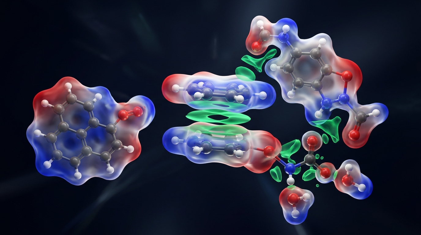
Mais de \(90\%\) de todos os cálculos quânticos publicados hoje em Química Orgânica, Catálise Homogénea e Heterogénea, Bioquímica Enzimática e Descoberta de Fármacos utilizam a Teoria do Funcional da Densidade (DFT). Contudo, na maioria dos livros de texto, a DFT é apresentada de forma demasiado matemática e abstrata, deixando o estudante sem saber como ligar os símbolos das equações às escolhas reais que tem de fazer no computador. Over \(90\%\) of all quantum calculations published today in Organic Chemistry, Homogeneous and Heterogeneous Catalysis, Enzymatic Biochemistry, and Drug Discovery rely on Density Functional Theory (DFT). Yet in most textbooks, DFT is presented in an overly abstract, mathematical way that leaves students unsure how to connect the symbols in the equations to the real choices they must make on the computer.
Por isso, desenhámos este capítulo especial como um livro dentro do livro: começamos na Secção 00 sem assumir qualquer pré-requisito avançado, usando paralelismos com montanhas, mapas topográficos, enxames de abelhas e recibos de restaurante antes de cada equação, até chegarmos aos cálculos reais em ORCA 5.0.3. We therefore designed this special chapter as a book within the book: starting in Section 00 without assuming any advanced prerequisites, using everyday parallels with mountains, topographic maps, honeybee swarms, and restaurant bills before every equation, all the way to real calculations in ORCA 5.0.3.
0.1 O Que Faz Realmente um Programa de Química Quântica? A Superfície de Energia Potencial \(E(\mathbf{R})\) 0.1 What Does a Quantum Chemistry Program Actually Do? The Potential Energy Surface \(E(\mathbf{R})\)
Imagine que os átomos de uma molécula são caminhantes numa cordilheira alpina onde a altitude do terreno em cada ponto é a Energia Total \(E(\mathbf{R})\). As moléculas estáveis (reagentes e produtos) vivem descansadas no fundo dos vales (onde o chão é plano e sobe em todas as direções). Para transformar reagentes em produtos, a molécula não sobe ao pico mais alto do Monte Evereste — ela procura o passo de montanha (colo ou sela) mais baixo entre os dois vales: o Estado de Transição (\(\ddagger\))! Imagine the atoms of a molecule as hikers in an alpine mountain range where the altitude of the terrain at every point is the Total Energy \(E(\mathbf{R})\). Stable molecules (reactants and products) rest at the bottom of valleys (where the ground is flat and curves upward in every direction). To turn reactants into products, a molecule does not climb to the top of Mount Everest — it seeks the lowest mountain pass (saddle point) between the two valleys: the Transition State (\(\ddagger\))!
Quando um estudante de Química, Bioquímica ou Ciências Farmacêuticas abre pela primeira vez um livro de Química Quântica, é fácil sentir-se perdido num mar de símbolos (\(\hat{H}\), \(\Psi\), \(\nabla^2\), \(\int d\tau\)) sem perceber para que serve tudo isto na prática. Por isso, comecemos pela visão global mais simples e poderosa de todas: When a Chemistry, Biochemistry, or Pharmaceutical Sciences student opens a Quantum Chemistry textbook for the first time, it is easy to feel lost in a sea of symbols (\(\hat{H}\), \(\Psi\), \(\nabla^2\), \(\int d\tau\)) without seeing what all of this is actually used for in practice. Let us therefore start with the simplest, most powerful big picture:
Ideia Fundamental Qualquer cálculo de estrutura eletrónica (seja Hartree–Fock, \(\text{CCSD(T)}\) ou \(\text{DFT}\)) funciona como uma caixa matemática universal: Core Idea Every electronic-structure calculation (whether Hartree–Fock, \(\text{CCSD(T)}\), or \(\text{DFT}\)) acts as a universal mathematical box:
- O que entra na caixa (Input):What goes into the box (Input): As coordenadas espaciais 3D \((X_A, Y_A, Z_A)\) e os números atómicos \(Z_A\) de todos os \(M\) núcleos da molécula (representados abreviadamente por \(\mathbf{R} = \{\mathbf{R}_1, \dots, \mathbf{R}_M\}\)), a carga elétrica total \(Q\) (que fixa o número total de eletrões \(N = \sum_{A=1}^M Z_A - Q\)) e a multiplicidade de spin \(2S + 1\) (que diz quantos eletrões estão desemparelhados). The 3D spatial coordinates \((X_A, Y_A, Z_A)\) and atomic numbers \(Z_A\) of all \(M\) nuclei in the molecule (denoted collectively as \(\mathbf{R} = \{\mathbf{R}_1, \dots, \mathbf{R}_M\}\)), the net electric charge \(Q\) (which fixes the total number of electrons \(N = \sum_{A=1}^M Z_A - Q\)), and the spin multiplicity \(2S + 1\) (which specifies how many electrons are unpaired).
- O que sai da caixa (Output):What comes out of the box (Output): A Energia Total \(E(\mathbf{R})\) dessa geometria molecular exata, juntamente com a distribuição espacial da sua nuvem eletrónica \(\rho(x,y,z)\)! The Total Energy \(E(\mathbf{R})\) of that exact molecular geometry, together with the spatial distribution of its electron cloud \(\rho(x,y,z)\)!
Se repetirmos este cálculo para diferentes posições dos núcleos \(\mathbf{R}\) (por exemplo, variando comprimentos de ligação e ângulos de torsão), a função \(E(\mathbf{R})\) desenha uma paisagem montanhosa multidimensional chamada Superfície de Energia Potencial (PES — Potential Energy Surface). Quase tudo o que um químico quer saber obtém-se calculando a altitude, a inclinação (primeira derivada) e a curvatura (segunda derivada) desta paisagem: If we repeat this calculation for different nuclear positions \(\mathbf{R}\) (for example, varying bond lengths and torsion angles), the function \(E(\mathbf{R})\) maps out a multidimensional mountain landscape called the Potential Energy Surface (PES). Almost everything a chemist wants to know is obtained from the altitude, slope (first derivative), and curvature (second derivative) of this landscape:
No fundo de um vale, a força sobre todos os átomos é nula (\(\mathbf{F}_A = \mathbf{0}\)) e a curvatura é positiva em todas as direções (\(0\) frequências imaginárias). É assim que o computador descobre a geometria 3D de uma molécula! At the bottom of a valley, the force on every atom is zero (\(\mathbf{F}_A = \mathbf{0}\)) and the curvature is positive in every direction (\(0\) imaginary frequencies). This is how the computer finds a molecule's 3D geometry!
No topo do passo de montanha mais baixo entre reagentes e produtos, \(\mathbf{g} = \mathbf{0}\), mas a superfície curva para baixo ao longo de uma única direção (a coordenada de reação), dando exatamente \(1\) frequência vibracional imaginária! At the lowest mountain pass between reactants and products, \(\mathbf{g} = \mathbf{0}\), but the surface curves downward along one single direction (the reaction coordinate), yielding exactly \(1\) imaginary vibrational frequency!
Combinando a energia eletrónica \(\Delta E^\ddagger\) com as vibrações da matriz Hessiana (energia de ponto zero \(\text{ZPE}\) e entropia \(S\)), obtemos \(\Delta G^\ddagger\) e a constante de velocidade \(k(T) = \frac{k_B T}{h}\exp(-\Delta G^\ddagger / RT)\)! Combining the electronic barrier \(\Delta E^\ddagger\) with the Hessian vibrations (zero-point energy \(\text{ZPE}\) and entropy \(S\)) gives \(\Delta G^\ddagger\) and the rate constant \(k(T) = \frac{k_B T}{h}\exp(-\Delta G^\ddagger / RT)\)!
0.2 A Aproximação de Born–Oppenheimer (1927): Porque Podemos Separar Eletrões e Núcleos? 0.2 The Born–Oppenheimer Approximation (1927): Why Can We Separate Electrons and Nuclei?
Imagine um enxame de abelhas ultrarrápidas (os eletrões leves) a voar em redor de dois elefantes muito lentos (os núcleos pesados). Sempre que um elefante dá um passo milimétrico para o lado, o enxame de abelhas reorganiza-se instantaneamente à volta da nova posição dos elefantes! Por isso, podemos calcular a nuvem das abelhas tratando os elefantes como se estivessem temporariamente congelados no espaço. Imagine a swarm of ultrafast honeybees (the light electrons) buzzing around two slow-moving elephants (the heavy nuclei). Whenever an elephant takes a tiny step, the swarm of bees rearranges instantaneously around the elephants' new positions! We can therefore compute the bee cloud while treating the elephants as temporarily frozen in space.
Uma molécula completa contém \(M\) núcleos de coordenadas \(\mathbf{R} = \{\mathbf{R}_1, \dots, \mathbf{R}_M\}\) e \(N\) eletrões de coordenadas \(\mathbf{r} = \{\mathbf{r}_1, \dots, \mathbf{r}_N\}\). O Hamiltoniano exato de toda a molécula inclui a energia cinética dos núcleos (\(\hat{T}_n\)), a energia cinética dos eletrões (\(\hat{T}_e\)) e todas as atrações e repulsões eletrostáticas de Coulomb entre as cargas: A complete molecule contains \(M\) nuclei at coordinates \(\mathbf{R} = \{\mathbf{R}_1, \dots, \mathbf{R}_M\}\) and \(N\) electrons at coordinates \(\mathbf{r} = \{\mathbf{r}_1, \dots, \mathbf{r}_N\}\). The exact molecular Hamiltonian includes the nuclear kinetic energy (\(\hat{T}_n\)), the electronic kinetic energy (\(\hat{T}_e\)), and all Coulomb attractions and repulsions between the charges:
Porque é que podemos resolver primeiro a equação apenas para os eletrões, mantendo os núcleos congelados (\(\hat{T}_n \to 0\))? Pela enorme disparidade de massas: Why can we solve the equation for the electrons first while holding the nuclei clamped (\(\hat{T}_n \to 0\))? Because of the enormous mass disparity:
- Um único protão (\(^1\text{H}\)) pesa \(m_p = 1836.15\,m_e\); um núcleo de Carbono (\(^{12}\text{C}\)) pesa \(\approx 21\,894\,m_e\); um núcleo de Ferro (\(^{56}\text{Fe}\)) pesa mais de \(102\,000\,m_e\)!A single proton (\(^1\text{H}\)) weighs \(m_p = 1836.15\,m_e\); a Carbon nucleus (\(^{12}\text{C}\)) weighs \(\approx 21\,894\,m_e\); an Iron nucleus (\(^{56}\text{Fe}\)) weighs over \(102\,000\,m_e\)!
- Como a energia cinética nuclear é \(\hat{T}_n = -\sum_{A=1}^M \frac{1}{2 M_A}\nabla_A^2\), o fator \(\frac{1}{M_A}\) é milhares de vezes mais pequeno do que nos eletrões. Os eletrões movem-se à escala de attosegundos (\(10^{-18}\text{ s}\)), enquanto as vibrações nucleares ocorrem à escala de femtossegundos a picossegundos (\(10^{-14}\text{ a }10^{-12}\text{ s}\)).Because nuclear kinetic energy is \(\hat{T}_n = -\sum_{A=1}^M \frac{1}{2 M_A}\nabla_A^2\), the prefactor \(\frac{1}{M_A}\) is thousands of times smaller than for electrons. Electrons move on the attosecond (\(10^{-18}\text{ s}\)) timescale, whereas nuclear vibrations occur on the femtosecond to picosecond (\(10^{-14}\text{ to }10^{-12}\text{ s}\)) timescale.
- Assim, para qualquer geometria fixa \(\mathbf{R}\), resolvemos \(\hat{H}_{\text{elec}}(\mathbf{r}; \mathbf{R})\Psi(\mathbf{r}; \mathbf{R}) = E_{\text{elec}}(\mathbf{R})\Psi(\mathbf{r}; \mathbf{R})\) e somamos no fim a repulsão eletrostática clássica entre os núcleos fixos: \(E_{\text{BO}}(\mathbf{R}) = E_{\text{elec}}(\mathbf{R}) + \sum_{A \lt B} \frac{Z_A Z_B}{|\mathbf{R}_A - \mathbf{R}_B|}\).Thus, at any fixed geometry \(\mathbf{R}\), we solve \(\hat{H}_{\text{elec}}(\mathbf{r}; \mathbf{R})\Psi(\mathbf{r}; \mathbf{R}) = E_{\text{elec}}(\mathbf{R})\Psi(\mathbf{r}; \mathbf{R})\) and add the classical repulsion between the fixed nuclei at the end: \(E_{\text{BO}}(\mathbf{R}) = E_{\text{elec}}(\mathbf{R}) + \sum_{A \lt B} \frac{Z_A Z_B}{|\mathbf{R}_A - \mathbf{R}_B|}\).
0.3 O Que É um Operador Quântico e Como Funcionam as 3 Parcelas de \(\hat{H}_{\text{elec}}\)? 0.3 What Is a Quantum Operator and How Do the 3 Pieces of \(\hat{H}_{\text{elec}}\) Work?
• Por exemplo, o operador de posição ou de energia potencial \(\hat{V}(\mathbf{r})\) dá uma instrução simples: «multiplique a função de onda \(\Psi(\mathbf{r})\) pelo valor do potencial \(V(\mathbf{r})\) em cada ponto!» (chama-se um operador multiplicativo local).
• Já o operador de energia cinética \(\hat{T}_e = -\frac{1}{2}\nabla^2\) dá uma instrução de derivação: «calcule a segunda derivada espacial (\(\frac{\partial^2}{\partial x^2} + \frac{\partial^2}{\partial y^2} + \frac{\partial^2}{\partial z^2}\)) da função de onda \(\Psi(\mathbf{r})\) e multiplique por \(-1/2\)!»
• E a notação \(\langle \Psi | \hat{H} | \Psi \rangle\) (chamada notação bra-ket de Paul Dirac) é apenas uma forma elegante e curta de escrever o integral da energia média em todo o espaço: $$\langle \Psi | \hat{H} | \Psi \rangle \equiv \int \Psi^*\,(\hat{H}\Psi)\,d\tau$$ Basta aplicar a instrução \(\hat{H}\) à função \(\Psi\), multiplicar por \(\Psi^*\) e somar (integrar) em todo o espaço! The "hat" (caret) denotes a Mathematical Operator — that is, a calculation instruction that acts on the function written to its right:
• For example, the potential energy operator \(\hat{V}(\mathbf{r})\) gives a simple instruction: "multiply the wavefunction \(\Psi(\mathbf{r})\) by the potential value \(V(\mathbf{r})\) at each point!" (this is called a local multiplicative operator).
• Meanwhile, the kinetic energy operator \(\hat{T}_e = -\frac{1}{2}\nabla^2\) gives a differentiation instruction: "take the second spatial derivative (\(\frac{\partial^2}{\partial x^2} + \frac{\partial^2}{\partial y^2} + \frac{\partial^2}{\partial z^2}\)) of \(\Psi(\mathbf{r})\) and multiply by \(-1/2\)!"
• And the notation \(\langle \Psi | \hat{H} | \Psi \rangle\) (called Paul Dirac's bra-ket notation) is simply a clean shorthand for the average-energy integral over all space: $$\langle \Psi | \hat{H} | \Psi \rangle \equiv \int \Psi^*\,(\hat{H}\Psi)\,d\tau$$ You simply apply the instruction \(\hat{H}\) to \(\Psi\), multiply by \(\Psi^*\), and integrate over all space!
Escrevendo explicitamente em Unidades Atómicas os três operadores do Hamiltoniano eletrónico para uma molécula com \(N\) eletrões e \(M\) núcleos, temos: Writing out the three operators of the electronic Hamiltonian explicitly in Atomic Units for a molecule with \(N\) electrons and \(M\) nuclei gives:
Repare na estrutura desta equação, pois toda a Teoria do Funcional da Densidade nasce de uma observação simples sobre ela: Look closely at the structure of this equation, because all of Density Functional Theory is born from one simple observation about it:
- Os operadores \(\hat{T}_e\) e \(\hat{V}_{ee}\) dependem apenas do número total de eletrões \(N\): são exatamente os mesmos para qualquer molécula com \(N\) eletrões (por exemplo, a molécula de água \(\text{H}_2\text{O}\), o metano \(\text{CH}_4\), o amoníaco \(\text{NH}_3\) e o átomo de Néon \(\text{Ne}\) têm todos \(N = 10\) eletrões, logo têm exatamente os mesmos operadores \(\hat{T}_e\) e \(\hat{V}_{ee}\)!).The operators \(\hat{T}_e\) and \(\hat{V}_{ee}\) depend only on the total number of electrons \(N\): they are identical for every \(N\)-electron system (for instance, water \(\text{H}_2\text{O}\), methane \(\text{CH}_4\), ammonia \(\text{NH}_3\), and the Neon atom \(\text{Ne}\) all have \(N = 10\) electrons, so they share the exact same \(\hat{T}_e\) and \(\hat{V}_{ee}\) operators!).
- A única coisa que distingue a água (\(\text{H}_2\text{O}\)) do metano (\(\text{CH}_4\)) é o potencial eletrostático externo dos núcleos, \(v_{\text{ext}}(\mathbf{r}) = -\sum_{A=1}^M \frac{Z_A}{|\mathbf{r} - \mathbf{R}_A|}\), que é uma simples função das 3 coordenadas do espaço \((x,y,z)\)!The only thing that distinguishes water (\(\text{H}_2\text{O}\)) from methane (\(\text{CH}_4\)) is the external electrostatic potential of the nuclei, \(v_{\text{ext}}(\mathbf{r}) = -\sum_{A=1}^M \frac{Z_A}{|\mathbf{r} - \mathbf{R}_A|}\), which is a simple function of the 3 spatial coordinates \((x,y,z)\)!
0.4 Unidades Atómicas, Teorema do Virial e a Escala da «Precisão Química» (\(1\text{ kcal/mol}\)) 0.4 Atomic Units, the Virial Theorem & the Scale of "Chemical Accuracy" (\(1\text{ kcal/mol}\))
Para consultar a qualquer momento durante a leitura deste capítulo e na resolução dos exercícios, guarde esta tabela de conversão entre as Unidades Atómicas (Hartree \(\text{E}_\text{h}\) e Bohr \(a_0\)) usadas pelos programas de Química Quântica e as unidades experimentais de laboratório: For quick reference throughout this chapter and when solving problems, keep this conversion table between the Atomic Units (Hartree \(\text{E}_\text{h}\) and Bohr \(a_0\)) used by Quantum Chemistry software and experimental laboratory units:
| Grandeza FísicaPhysical Quantity | Símbolo e Nome em Unidades AtómicasAtomic Unit Symbol & Name | Equivalência em Unidades Químicas e SIEquivalence in Chemical & SI Units | Referência Física no Átomo de Hidrogénio (\(\text{1s}^1\))Physical Reference in the Hydrogen Atom (\(\text{1s}^1\)) |
|---|---|---|---|
| Distância / ComprimentoLength / Distance | \(1\,a_0\) (1 Bohr) | \(\mathbf{0.529177\text{ Å}} = 52.918\text{ pm}\) | Raio mais provável da orbital \(\text{1s}\) do átomo de \(\text{H}\).Most probable radius of the \(\text{H}\) atom \(\text{1s}\) orbital. |
| EnergiaEnergy | \(1\text{ E}_\text{h}\) (1 Hartree) | \(\mathbf{627.5095\text{ kcal/mol}} = 2625.50\text{ kJ/mol} = 27.2114\text{ eV}\) | A energia exata do átomo de \(\text{H}\) no estado fundamental é \(E_{\text{H}} = -\frac{1}{2}\text{ E}_\text{h} = -0.500000\text{ E}_\text{h}\) (\(-313.75\text{ kcal/mol}\)).The exact ground-state energy of the \(\text{H}\) atom is \(E_{\text{H}} = -\frac{1}{2}\text{ E}_\text{h} = -0.500000\text{ E}_\text{h}\) (\(-313.75\text{ kcal/mol}\)). |
| «Precisão Química»"Chemical Accuracy" | \(0.001594\text{ E}_\text{h} \approx 1.6\text{ mE}_\text{h}\) | \(\mathbf{1.00\text{ kcal/mol}} = 4.184\text{ kJ/mol} = 0.0434\text{ eV}\) | Meta de exatidão termoquímica: a \(298\text{ K}\), um erro de \(1.36\text{ kcal/mol}\) altera uma constante de equilíbrio \(K_{\text{eq}}\) em \(10\times\)!Thermochemical accuracy target: at \(298\text{ K}\), a \(1.36\text{ kcal/mol}\) error shifts an equilibrium constant \(K_{\text{eq}}\) by \(10\times\)! |
Objetivo: Converter diferenças de energia entre Hartree (\(\text{E}_\text{h}\)), milihartree (\(\text{mE}_\text{h}\)), \(\text{kcal/mol}\), \(\text{kJ/mol}\) e \(\text{eV}\), e visualizar o impacto exponencial de qualquer erro energético nas constantes de equilíbrio e velocidade a \(298.15\text{ K}\). Goal: Convert energy differences among Hartree (\(\text{E}_\text{h}\)), millihartree (\(\text{mE}_\text{h}\)), \(\text{kcal/mol}\), \(\text{kJ/mol}\), and \(\text{eV}\), and visualize the exponential impact of any energy error on equilibrium and rate constants at \(298.15\text{ K}\).
ℹ️ Explicação deste seletor / controlo (clique para abrir)ℹ️ Explanation of this selector / control (click to open)
ℹ️ Explicação deste seletor / controlo (clique para abrir)ℹ️ Explanation of this selector / control (click to open)
Se a Equação de Schrödinger \(\hat{H}_{\text{elec}}\Psi = E_{\text{elec}}\Psi\) já é conhecida exatamente desde 1926, porque é que não a resolvemos diretamente para uma proteína ou para um fármaco? Na Secção 01 vamos descobrir a chamada «Parede Exponencial» da função de onda \(\Psi(\mathbf{x}_1, \dots, \mathbf{x}_N)\) e ver como a densidade eletrónica 3D \(\rho(x,y,z)\) nos oferece uma saída extraordinária! If the Schrödinger Equation \(\hat{H}_{\text{elec}}\Psi = E_{\text{elec}}\Psi\) has been known exactly since 1926, why can't we solve it directly for a protein or a drug molecule? In Section 01 we will uncover the "Exponential Wall" of the many-electron wavefunction \(\Psi(\mathbf{x}_1, \dots, \mathbf{x}_N)\) and see how the 3D electron density \(\rho(x,y,z)\) offers an extraordinary way out!
Verifique os conceitos fundamentais desta secção do Capítulo 16 (DFT) e veja o que deve estudar mais.Check your grasp of the fundamental concepts of this Chapter 16 (DFT) section and see what to study further.
O Problema de Muitos Eletrões: Da Função de Onda Antissimétrica \(\Psi\) (\(4N\) Variáveis) à Densidade Eletrónica 3D \(\rho(\mathbf{r})\) The Many-Electron Problem: From the Antisymmetric Wavefunction \(\Psi\) (\(4N\) Variables) to the 3D Electron Density \(\rho(\mathbf{r})\)
Compreender o spin eletrónico, o Determinante de Slater, a parede exponencial dos métodos de função de onda e como a densidade \(\rho(x,y,z)\) codifica toda a molécula em apenas 3 dimensões. Understanding electron spin, the Slater Determinant, the exponential wall of wavefunction methods, and how the density \(\rho(x,y,z)\) encodes the entire molecule in just 3 dimensions.
Na Secção 00 vimos que, uma vez fixados os núcleos pela aproximação de Born–Oppenheimer, só precisamos de encontrar a energia dos \(N\) eletrões. Para \(1\) único eletrão (átomo de Hidrogénio), a função de onda \(\psi(x,y,z)\) vive no nosso espaço familiar de \(3\) dimensões. Mas o que acontece quando passamos para uma molécula de água (\(10\) eletrões), um comprimido de Aspirina (\(94\) eletrões) ou uma enzima (\(25\,000\) eletrões)? Vamos ver porque é que a função de onda \(\Psi\) choca contra uma «Parede Exponencial» — e como a densidade eletrónica 3D \(\rho(x,y,z)\) derruba essa parede! In Section 00 we saw that once the nuclei are clamped via the Born–Oppenheimer approximation, we only need to find the energy of the \(N\) electrons. For a single electron (Hydrogen atom), the wavefunction \(\psi(x,y,z)\) lives in our familiar \(3\)-dimensional space. What happens when we move to a water molecule (\(10\) electrons), an Aspirin tablet (\(94\) electrons), or an enzyme (\(25\,000\) electrons)? Let us see why the wavefunction \(\Psi\) hits an "Exponential Wall" — and how the 3D electron density \(\rho(x,y,z)\) breaks right through it!
1.1 Spin Eletrónico, o Princípio da Antissimetria de Pauli e o Determinante de Slater 1.1 Electron Spin, Pauli's Antisymmetry Principle & the Slater Determinant
Passo 1 Para descrever completamente um eletrão \(i\), não basta indicar as suas 3 coordenadas espaciais \(\mathbf{r}_i = (x_i, y_i, z_i)\); temos também de indicar a sua coordenada interna de spin \(\sigma_i\), que pode assumir dois estados quânticos: \(\alpha\) (\(\uparrow\), \(m_s = +\frac{1}{2}\)) ou \(\beta\) (\(\downarrow\), \(m_s = -\frac{1}{2}\)). Juntando espaço e spin numa única notação \(\mathbf{x}_i \equiv (\mathbf{r}_i, \sigma_i)\), a função de onda de uma molécula com \(N\) eletrões escreve-se \(\Psi(\mathbf{x}_1, \mathbf{x}_2, \dots, \mathbf{x}_N)\). Step 1 To completely describe an electron \(i\), specifying its 3 spatial coordinates \(\mathbf{r}_i = (x_i, y_i, z_i)\) is not enough; we must also specify its internal spin coordinate \(\sigma_i\), which can take two quantum states: \(\alpha\) (\(\uparrow\), \(m_s = +\frac{1}{2}\)) or \(\beta\) (\(\downarrow\), \(m_s = -\frac{1}{2}\)). Combining space and spin into a single label \(\mathbf{x}_i \equiv (\mathbf{r}_i, \sigma_i)\), the wavefunction of an \(N\)-electron molecule is written \(\Psi(\mathbf{x}_1, \mathbf{x}_2, \dots, \mathbf{x}_N)\).
Passo 2 Como os eletrões são partículas de spin semi-inteiro (\(s = 1/2\), chamados fermiões) e são fisicamente indistinguíveis uns dos outros, Wolfgang Pauli descobriu em 1925 uma lei fundamental da Natureza — o Princípio da Antissimetria de Pauli: se trocarmos as coordenadas completas \((\mathbf{x}_i \leftrightarrow \mathbf{x}_j)\) de quaisquer dois eletrões, a função de onda tem obrigatoriamente de mudar de sinal! Step 2 Because electrons are half-integer spin particles (\(s = 1/2\), called fermions) and are physically indistinguishable from one another, Wolfgang Pauli discovered in 1925 a fundamental law of Nature — Pauli's Antisymmetry Principle: if we swap the complete coordinates \((\mathbf{x}_i \leftrightarrow \mathbf{x}_j)\) of any two electrons, the wavefunction must change sign!
Repare no que acontece se tentarmos colocar dois eletrões com o mesmo spin (\(\sigma_1 = \sigma_2\)) no mesmo ponto do espaço (\(\mathbf{r}_1 = \mathbf{r}_2\)), ou seja, \(\mathbf{x}_1 = \mathbf{x}_2\): as duas linhas do determinante ficam exatamente iguais e \(\Phi_{\text{SD}}(\mathbf{x}_1, \mathbf{x}_1) = \frac{1}{\sqrt{2}}\left[\chi_1(\mathbf{x}_1)\chi_2(\mathbf{x}_1) - \chi_1(\mathbf{x}_1)\chi_2(\mathbf{x}_1)\right] = \mathbf{0}\)! Isto significa que a probabilidade de encontrar dois eletrões de mesmo spin no mesmo sítio é automaticamente zero! É esta propriedade matemática que cria o chamado Buraco de Troca (ou Buraco de Fermi) e a Energia de Troca \(E_{\text{X}}\) que estudaremos nas Secções 3 e 4! Notice what happens if we try to place two electrons of the same spin (\(\sigma_1 = \sigma_2\)) at the same point in space (\(\mathbf{r}_1 = \mathbf{r}_2\)), so that \(\mathbf{x}_1 = \mathbf{x}_2\): the two rows of the determinant become identical and \(\Phi_{\text{SD}}(\mathbf{x}_1, \mathbf{x}_1) = \frac{1}{\sqrt{2}}\left[\chi_1(\mathbf{x}_1)\chi_2(\mathbf{x}_1) - \chi_1(\mathbf{x}_1)\chi_2(\mathbf{x}_1)\right] = \mathbf{0}\)! This means the probability of finding two parallel-spin electrons at the same point in space is automatically zero! This mathematical property creates the Exchange Hole (or Fermi Hole) and the Exchange Energy \(E_{\text{X}}\) that we will study in Sections 3 and 4!
1.2 A «Parede Exponencial» de Walter Kohn e a Escalabilidade dos Métodos Quânticos 1.2 Walter Kohn's "Exponential Wall" and the Scaling of Quantum Methods
Seguir a função de onda \(\Psi(\mathbf{r}_1, \dots, \mathbf{r}_N)\) de uma proteína com \(25\,000\) eletrões é como tentar anotar em simultâneo a posição instantânea acoplada de \(25\,000\) automóveis em Lisboa: se guardarmos apenas \(10\) pontos por eixo, precisaríamos de \(10^{75\,000}\) números (há apenas \(\sim 10^{80}\) átomos em todo o Universo visível!). Já a densidade eletrónica \(\rho(x,y,z)\) funciona como o mapa de calor de trânsito no telemóvel: independentemente de estarem \(2\), \(94\) ou \(25\,000\) carros na cidade, o mapa tem sempre apenas 3 coordenadas \((x, y, z)\)! Tracking the wavefunction \(\Psi(\mathbf{r}_1, \dots, \mathbf{r}_N)\) of a protein with \(25\,000\) electrons is like trying to record the simultaneous coupled positions of \(25\,000\) cars in a city: with just \(10\) grid points per axis, we would need \(10^{75\,000}\) numbers (there are only \(\sim 10^{80}\) atoms in the entire observable Universe!). By contrast, the electron density \(\rho(x,y,z)\) works like the traffic heat map on your phone: whether there are \(2\), \(94\), or \(25\,000\) cars in the city, the map always has just 3 spatial coordinates \((x, y, z)\)!
No seu discurso de aceitação do Prémio Nobel da Química em 1998, Walter Kohn chamou «Parede Exponencial» (Exponential Wall) à impossibilidade de representar diretamente a função de onda \(\Psi(\mathbf{x}_1, \dots, \mathbf{x}_N)\) de \(3N\) coordenadas espaciais quando \(N\) cresce. Compare na tabela abaixo como o tempo de cálculo cresce quando duplicamos o tamanho da molécula (\(N \to 2N\)) nos diferentes métodos da Química Quântica: In his 1998 Nobel Prize lecture, Walter Kohn coined the term "Exponential Wall" for the impossibility of directly representing the \(3N\)-coordinate wavefunction \(\Psi(\mathbf{x}_1, \dots, \mathbf{x}_N)\) as \(N\) grows. Compare in the table below how computer time grows when we double the size of a molecule (\(N \to 2N\)) across Quantum Chemistry methods:
| Método QuânticoQuantum Method | Variável FundamentalFundamental Variable | Escalonamento FormalFormal Scaling | Se duplicar a molécula (\(2\times\)), o tempo multiplica por:If molecule size doubles (\(2\times\)), runtime multiplies by: | Limite Prático Típico (N.º de Átomos)Typical Practical Limit (Atoms) |
|---|---|---|---|---|
| DFT Semilocal (GGA / meta-GGA com RI-J)Semilocal DFT (GGA / meta-GGA with RI-J) | Densidade 3D \(\rho(x,y,z)\) + \(N\) orbitais KS3D Density \(\rho(x,y,z)\) + \(N\) KS orbitals | \(\mathcal{O}(N^3)\) | \(2^3 = 8\times\) | \(200\text{ a }2\,000\) átomos\(200\text{ to }2,000\) atoms |
DFT Híbrida (ex.: B3LYP, ωB97X-D3 com RIJCOSX)Hybrid DFT (e.g., B3LYP, ωB97X-D3 with RIJCOSX) |
Densidade 3D \(\rho(x,y,z)\) + orbitais KS + troca HF3D Density \(\rho(x,y,z)\) + KS orbitals + HF exchange | \(\mathcal{O}(N^3\text{–}N^4)\) | \(8\times\text{ a }16\times\)\(8\times\text{ to }16\times\) | \(100\text{ a }800\) átomos\(100\text{ to }800\) atoms |
MP2 / Duplos Híbridos (ex.: B2PLYP)MP2 / Double Hybrids (e.g., B2PLYP) |
Orbitais ocupadas e virtuais (excitações duplas)Occupied & virtual orbitals (double excitations) | \(\mathcal{O}(N^5)\) | \(2^5 = 32\times\) | \(50\text{ a }200\) átomos\(50\text{ to }200\) atoms |
| CCSD(T) («Padrão de Ouro» Canónico)CCSD(T) (Canonical "Gold Standard") | Função de onda correlacionada \(\hat{T}_1, \hat{T}_2, (\hat{T}_3)\)Correlated wavefunction \(\hat{T}_1, \hat{T}_2, (\hat{T}_3)\) | \(\mathcal{O}(N^7)\) | \(2^7 = 128\times\)! | \(15\text{ a }35\) átomos (ou mais com DLPNO)\(15\text{ to }35\) atoms (or more with DLPNO) |
| Full CI (Solução Exata na Base)Full CI (Exact Solution in Basis) | Todos os determinantes possíveis \(\binom{2K}{N}\)All possible determinants \(\binom{2K}{N}\) | \(\mathcal{O}(N!)\) | Exponencial!Exponential! | \(\lt 6\) átomos (\(\sim 14\text{–}18\) eletrões)\(\lt 6\) atoms (\(\sim 14\text{–}18\) electrons) |
1.3 A Densidade Eletrónica 3D \(\rho(\mathbf{r})\) e a Densidade de Spin \(\rho_s(\mathbf{r})\) 1.3 The 3D Electron Density \(\rho(\mathbf{r})\) and the Spin Density \(\rho_s(\mathbf{r})\)
Na DFT moderna (chamada Spin-DFT), distinguimos a densidade dos eletrões de spin \(\alpha\) (\(\uparrow\)), \(\rho_\alpha(\mathbf{r})\), e a densidade dos eletrões de spin \(\beta\) (\(\downarrow\)), \(\rho_\beta(\mathbf{r})\). Com elas formamos duas funções tridimensionais com enorme valor químico: In modern DFT (called Spin-DFT), we distinguish the density of \(\alpha\)-spin (\(\uparrow\)) electrons, \(\rho_\alpha(\mathbf{r})\), and the density of \(\beta\)-spin (\(\downarrow\)) electrons, \(\rho_\beta(\mathbf{r})\). From these we form two 3D functions of immense chemical value:
Numa molécula de camada fechada (como a água \(\text{H}_2\text{O}\) ou o dímero de árgon \(\text{Ar}_2\)), todos os eletrões estão emparelhados (\(\rho_\alpha(\mathbf{r}) = \rho_\beta(\mathbf{r}) = \frac{1}{2}\rho(\mathbf{r})\)), logo a densidade de spin \(\rho_s(\mathbf{r})\) é zero em todo o espaço. Já num radical livre (como o estado de transição \([\text{H}\cdots\text{H}\cdots\text{H}]^\ddagger\) com \(N_\alpha = 2\) e \(N_\beta = 1\)) ou num centro metálico enzimático de Ferro ou Cobre, o mapa 3D de \(\rho_s(\mathbf{r})\) mostra exatamente em que átomos está localizado o eletrão desemparelhado! In a closed-shell molecule (like water \(\text{H}_2\text{O}\) or the argon dimer \(\text{Ar}_2\)), all electrons are paired (\(\rho_\alpha(\mathbf{r}) = \rho_\beta(\mathbf{r}) = \frac{1}{2}\rho(\mathbf{r})\)), so the spin density \(\rho_s(\mathbf{r})\) vanishes everywhere. In a free radical (like the transition state \([\text{H}\cdots\text{H}\cdots\text{H}]^\ddagger\) with \(N_\alpha = 2\) and \(N_\beta = 1\)) or an enzymatic Iron or Copper center, the 3D map of \(\rho_s(\mathbf{r})\) directly reveals which atoms host the unpaired electron!
1.4 Como a Densidade \(\rho(\mathbf{r})\) Codifica Toda a Molécula: Cúspide Nuclear de Kato e Decaimento Assintótico 1.4 How the Density \(\rho(\mathbf{r})\) Encodes the Entire Molecule: Kato's Nuclear Cusp & Asymptotic Decay
Objetivo: Compreender a revolução do 1.º Teorema de Hohenberg–Kohn: comparar a explosão dimensional da função de onda \(\Psi(3N\text{ coordenadas})\) com a simplicidade da densidade eletrónica \(\rho(x,y,z)\) (sempre \(3\) coordenadas!) e observar como a Cúspide de Kato nos núcleos codifica o número atómico \(Z_A\). Goal: Grasp the revolution of the 1st Hohenberg–Kohn Theorem: contrast the dimensional explosion of the wavefunction \(\Psi(3N\text{ coordinates})\) against the \(3\)-coordinate electron density \(\rho(x,y,z)\), and see how Kato's nuclear cusp encodes the atomic number \(Z_A\).
ℹ️ Explicação deste seletor / controlo (clique para abrir)ℹ️ Explanation of this selector / control (click to open)
ℹ️ Explicação deste seletor / controlo (clique para abrir)ℹ️ Explanation of this selector / control (click to open)
Parece impossível, mas a densidade guarda tudo o que é preciso para reconstruir o Hamiltoniano. O integral \(\int \rho(\mathbf{r})\,d\mathbf{r}\) dá o número de eletrões \(N\). As cúspides (pontas) da densidade dizem onde estão os núcleos, e o declive de cada cúspide dá a carga nuclear \(Z\) (Teorema de Kato). Com \(N\), as posições e as cargas, o Hamiltoniano fica completamente definido, e portanto tudo o resto também. O "preço" desta compressão é que a fórmula exata que liga \(\rho\) à energia não é conhecida e tem de ser aproximada, como veremos na Secção 2.It seems impossible, but the density stores everything needed to rebuild the Hamiltonian. The integral \(\int \rho(\mathbf{r})\,d\mathbf{r}\) gives the number of electrons \(N\). The cusps (sharp peaks) of the density show where the nuclei are, and the slope of each cusp gives the nuclear charge \(Z\) (Kato's Theorem). With \(N\), the positions, and the charges, the Hamiltonian is fully defined, and therefore so is everything else. The "price" of this compression is that the exact formula linking \(\rho\) to the energy is unknown and must be approximated, as we will see in Section 2.
Ao comprimirmos uma função de onda de \(3N\) dimensões numa nuvem de apenas \(3\) dimensões, não teremos perdido informação essencial sobre os eletrões? Na Secção 02 vamos ver como Pierre Hohenberg e Walter Kohn provaram em 1964, numa demonstração de quatro linhas de tirar o fôlego, que não se perde absolutamente nada no estado fundamental! By compressing a \(3N\)-dimensional wavefunction into a \(3\)-dimensional cloud, haven't we lost essential information about the electrons? In Section 02 we will see how Pierre Hohenberg and Walter Kohn proved in 1964, in a breathtaking four-line proof, that nothing at all is lost in the ground state!
Verifique os conceitos fundamentais desta secção do Capítulo 16 (DFT) e veja o que deve estudar mais.Check your grasp of the fundamental concepts of this Chapter 16 (DFT) section and see what to study further.
O Conceito de Funcional, Derivadas Funcionais, os Dois Teoremas de Hohenberg–Kohn (1964) e a Pesquisa de Levy–Lieb (1979) The Concept of a Functional, Functional Derivatives, the Two Hohenberg–Kohn Theorems (1964) & the Levy–Lieb Search (1979)
Dominar sem medo a matemática dos funcionais e acompanhar passo a passo as demonstrações que formam o alicerce da DFT moderna. Mastering the mathematics of functionals without fear and following step by step the proofs that form the bedrock of modern DFT.
Na Secção 01 vimos que a densidade \(\rho(x,y,z)\) é uma nuvem tridimensional muito mais simples do que a função de onda \(\Psi\). Mas para transformar essa nuvem num número — a Energia Total da molécula \(E[\rho]\) — precisamos de uma máquina matemática chamada Funcional. Vamos começar por perceber este conceito através de uma ida ao supermercado antes de seguirmos, passo a passo, os célebres teoremas de Hohenberg–Kohn e Levy–Lieb! In Section 01 we saw that the density \(\rho(x,y,z)\) is a three-dimensional cloud vastly simpler than the wavefunction \(\Psi\). To turn that entire cloud into a single number — the molecule's Total Energy \(E[\rho]\) — we need a mathematical machine called a Functional. Let us start by understanding this concept through a trip to the supermarket before walking step by step through the celebrated Hohenberg–Kohn and Levy–Lieb theorems!
2.1 Matemática Explicada do Zero: Funções \(f(x)\), Funcionais \(F[\rho]\) e Derivadas Funcionais \(\frac{\delta F[\rho]}{\delta \rho(\mathbf{r})}\) 2.1 Mathematics Explained from Scratch: Functions \(f(x)\), Functionals \(F[\rho]\) & Functional Derivatives \(\frac{\delta F[\rho]}{\delta \rho(\mathbf{r})}\)
Uma função \(p(x)\) é como a etiqueta de preço na prateleira: entra um código de produto \(x\) e sai o preço desse produto. Já um funcional \(F[\rho]\) é como a caixa registadora no fim das compras: entra a sua lista de compras inteira \(\rho(x)\) (quantos quilos levou de cada alimento) e sai um único número no talão: o Total a Pagar em Euros! E o que é a derivada funcional \(\delta F / \delta \rho(x)\)? É simplesmente responder: «Se eu acrescentar mais uma grama do produto \(x\) ao cesto, quantos cêntimos sobe a conta final?» A function \(p(x)\) is like a shelf price tag: input one item code \(x\) and out comes that item's price. By contrast, a functional \(F[\rho]\) is like the checkout register at the end of your shopping trip: input your entire shopping cart \(\rho(x)\) (how much of every item you bought) and out comes one single number on the receipt: the Total Bill! And what is the functional derivative \(\delta F / \delta \rho(x)\)? It simply answers: "If I add one extra gram of item \(x\) to the cart, by how many cents does the total bill go up?"
Para compreender as equações da DFT de forma cristalina, só precisa de distinguir três conceitos muito intuitivos: To understand the equations of DFT with crystal clarity, you only need to distinguish three very intuitive concepts:
- Função \(f(x)\) (parênteses curvos):Function \(f(x)\) (round parentheses): Recebe um número (ou ponto \(\mathbf{r}=(x,y,z)\)) e devolve um número. A densidade eletrónica \(\rho(\mathbf{r})\) é uma função da posição no espaço. Takes a number (or point \(\mathbf{r}=(x,y,z)\)) and returns a number. The electron density \(\rho(\mathbf{r})\) is a function of position in space.
- Funcional \(F[\rho]\) (parênteses retos):Functional \(F[\rho]\) (square brackets): Recebe uma função inteira \(\rho(\mathbf{r})\) e devolve um único número! Por exemplo, o número total de eletrões \(N[\rho] = \int \rho(\mathbf{r})\,d\mathbf{r}\) é um funcional da densidade, e a energia de atração núcleo–eletrão \(V_{ne}[\rho] = \int v_{\text{ext}}(\mathbf{r})\rho(\mathbf{r})\,d\mathbf{r}\) também é um funcional de \(\rho\)! Takes an entire function \(\rho(\mathbf{r})\) and returns a single number! For example, the total electron count \(N[\rho] = \int \rho(\mathbf{r})\,d\mathbf{r}\) is a functional of the density, and the nucleus–electron attraction energy \(V_{ne}[\rho] = \int v_{\text{ext}}(\mathbf{r})\rho(\mathbf{r})\,d\mathbf{r}\) is also a functional of \(\rho\)!
- Derivada Funcional \(\frac{\delta F[\rho]}{\delta \rho(\mathbf{r})}\) (com o símbolo \(\delta\)):Functional Derivative \(\frac{\delta F[\rho]}{\delta \rho(\mathbf{r})}\) (with the \(\delta\) symbol): Responde à pergunta: «Se adicionarmos uma gotícula minúscula de densidade \(\delta\rho(\mathbf{r})\) no ponto \(\mathbf{r}\), quanto muda o valor do funcional \(F[\rho]\)?» Ou seja, a derivada funcional de uma energia em ordem à densidade é um potencial elétrico sentido no ponto \(\mathbf{r}\)! Answers the question: "If we add a tiny droplet of density \(\delta\rho(\mathbf{r})\) at point \(\mathbf{r}\), how much does the functional \(F[\rho]\) change?" In other words, the functional derivative of an energy with respect to the density is an effective potential felt at point \(\mathbf{r}\)!
Por definição, a derivada funcional \(\frac{\delta F[\rho]}{\delta \rho(\mathbf{r})}\) é a função que multiplica \(\delta\rho(\mathbf{r})\) dentro do integral da variação linear \(\delta F = F[\rho + \delta\rho] - F[\rho] = \int \left(\frac{\delta F[\rho]}{\delta \rho(\mathbf{r})}\right)\delta\rho(\mathbf{r})\,d\mathbf{r}\). Veja como é fácil para os dois termos eletrostáticos da molécula: By definition, the functional derivative \(\frac{\delta F[\rho]}{\delta \rho(\mathbf{r})}\) is the function multiplying \(\delta\rho(\mathbf{r})\) inside the first-order variation integral \(\delta F = F[\rho + \delta\rho] - F[\rho] = \int \left(\frac{\delta F[\rho]}{\delta \rho(\mathbf{r})}\right)\delta\rho(\mathbf{r})\,d\mathbf{r}\). See how easy this is for the two electrostatic terms of a molecule:
$$\begin{gathered} \text{Exemplo 1 (Atração Núcleo–Eletrão): } V_{ne}[\rho] = \int v_{\text{ext}}(\mathbf{r})\,\rho(\mathbf{r})\,d\mathbf{r} \\[6pt] \implies\; \delta V_{ne} = \int v_{\text{ext}}(\mathbf{r})\,\delta\rho(\mathbf{r})\,d\mathbf{r} \\[6pt] \implies\; \frac{\delta V_{ne}[\rho]}{\delta \rho(\mathbf{r})} = v_{\text{ext}}(\mathbf{r}) \end{gathered}$$ $$\begin{gathered} \text{Exemplo 2 (Repulsão Clássica de Coulomb): } J[\rho] = \frac{1}{2}\iint \frac{\rho(\mathbf{r})\,\rho(\mathbf{r}')}{|\mathbf{r} - \mathbf{r}'|}\,d\mathbf{r}\,d\mathbf{r}' \\[6pt] \implies\; \frac{\delta J[\rho]}{\delta \rho(\mathbf{r})} = \int \frac{\rho(\mathbf{r}')}{|\mathbf{r} - \mathbf{r}'|}\,d\mathbf{r}' \equiv v_J(\mathbf{r}) \end{gathered}$$ $$\begin{gathered} \text{Example 1 (Nucleus–Electron Attraction): } V_{ne}[\rho] = \int v_{\text{ext}}(\mathbf{r})\,\rho(\mathbf{r})\,d\mathbf{r} \\[6pt] \implies\; \delta V_{ne} = \int v_{\text{ext}}(\mathbf{r})\,\delta\rho(\mathbf{r})\,d\mathbf{r} \\[6pt] \implies\; \frac{\delta V_{ne}[\rho]}{\delta \rho(\mathbf{r})} = v_{\text{ext}}(\mathbf{r}) \end{gathered}$$ $$\begin{gathered} \text{Example 2 (Classical Coulomb Repulsion): } J[\rho] = \frac{1}{2}\iint \frac{\rho(\mathbf{r})\,\rho(\mathbf{r}')}{|\mathbf{r} - \mathbf{r}'|}\,d\mathbf{r}\,d\mathbf{r}' \\[6pt] \implies\; \frac{\delta J[\rho]}{\delta \rho(\mathbf{r})} = \int \frac{\rho(\mathbf{r}')}{|\mathbf{r} - \mathbf{r}'|}\,d\mathbf{r}' \equiv v_J(\mathbf{r}) \end{gathered}$$ Repare que o fator \(1/2\) em \(J[\rho]\) cancela com o fator \(2\) que desce ao derivar \(\rho(\mathbf{r})\rho(\mathbf{r}')\), dando exatamente o potencial eletrostático clássico de Hartree \(v_J(\mathbf{r})\)! Da mesma forma, a derivada funcional da energia de troca-correlação define o potencial de troca-correlação: \(v_{\text{XC}}(\mathbf{r}) \equiv \frac{\delta E_{\text{XC}}[\rho]}{\delta \rho(\mathbf{r})}\). Notice how the factor of \(1/2\) in \(J[\rho]\) cancels the factor of \(2\) from differentiating \(\rho(\mathbf{r})\rho(\mathbf{r}')\), yielding the exact classical Hartree electrostatic potential \(v_J(\mathbf{r})\)! In the exact same way, the functional derivative of the exchange-correlation energy defines the exchange-correlation potential: \(v_{\text{XC}}(\mathbf{r}) \equiv \frac{\delta E_{\text{XC}}[\rho]}{\delta \rho(\mathbf{r})}\).2.2 Primeiro Teorema de Hohenberg–Kohn (1964) — Com Demonstração Passo a Passo 2.2 First Hohenberg–Kohn Theorem (1964) — With Step-by-Step Proof
Enunciado do 1.º Teorema de Hohenberg–Kohn: A densidade eletrónica do estado fundamental \(\rho_0(\mathbf{r})\) de um sistema de eletrões interagentes determina univocamente o potencial externo \(v_{\text{ext}}(\mathbf{r})\) (a menos de uma constante aditiva trivial). Statement of the 1st Hohenberg–Kohn Theorem: The ground-state electron density \(\rho_0(\mathbf{r})\) of a system of interacting electrons uniquely determines the external potential \(v_{\text{ext}}(\mathbf{r})\) (up to a trivial additive constant).
- Hipótese por redução ao absurdo: Suponhamos que existiam dois potenciais externos diferentes \(v_{\text{ext}}(\mathbf{r})\) e \(v'_{\text{ext}}(\mathbf{r})\) (que diferem por mais do que uma constante) capazes de produzir exatamente a mesma densidade eletrónica do estado fundamental \(\rho_0(\mathbf{r})\). Assumption for contradiction (reductio ad absurdum): Suppose two different external potentials \(v_{\text{ext}}(\mathbf{r})\) and \(v'_{\text{ext}}(\mathbf{r})\) (differing by more than a constant) could produce the exact same ground-state electron density \(\rho_0(\mathbf{r})\).
- Dois Hamiltonianos e duas funções de onda: Como \(v_{\text{ext}} \neq v'_{\text{ext}}\), os dois sistemas têm Hamiltonianos diferentes (\(\hat{H} = \hat{T}_e + \hat{V}_{ee} + \hat{V}_{\text{ext}}\) e \(\hat{H}' = \hat{T}_e + \hat{V}_{ee} + \hat{V}'_{\text{ext}}\)) e, portanto, funções de onda do estado fundamental diferentes, \(\Psi_0 \neq \Psi'_0\), com energias \(E_0\) e \(E'_0\). Two Hamiltonians and two wavefunctions: Because \(v_{\text{ext}} \neq v'_{\text{ext}}\), the two systems have different Hamiltonians (\(\hat{H} = \hat{T}_e + \hat{V}_{ee} + \hat{V}_{\text{ext}}\) and \(\hat{H}' = \hat{T}_e + \hat{V}_{ee} + \hat{V}'_{\text{ext}}\)) and therefore different ground-state wavefunctions, \(\Psi_0 \neq \Psi'_0\), with energies \(E_0\) and \(E'_0\).
- Aplicar o Princípio Variacional ao sistema 1 usando \(\Psi'_0\) como função tentativa: Como \(\Psi_0\) é o estado fundamental verdadeiro de \(\hat{H}\), qualquer outra função \(\Psi'_0\) dá uma energia estritamente maior. E como \(\hat{H} = \hat{H}' + \hat{V}_{\text{ext}} - \hat{V}'_{\text{ext}}\) e ambos os estados têm a mesma densidade \(\rho_0(\mathbf{r})\): Apply the Variational Principle to system 1 using \(\Psi'_0\) as a trial wavefunction: Because \(\Psi_0\) is the true ground state of \(\hat{H}\), any other wavefunction \(\Psi'_0\) gives a strictly higher energy. Using \(\hat{H} = \hat{H}' + \hat{V}_{\text{ext}} - \hat{V}'_{\text{ext}}\) and the assumed shared density \(\rho_0(\mathbf{r})\): $$\begin{gathered} E_0 = \langle \Psi_0 | \hat{H} | \Psi_0 \rangle < \langle \Psi'_0 | \hat{H} | \Psi'_0 \rangle \\[6pt] = \langle \Psi'_0 | \hat{H}' + \hat{V}_{\text{ext}} - \hat{V}'_{\text{ext}} | \Psi'_0 \rangle = E'_0 + \int \left[v_{\text{ext}}(\mathbf{r}) - v'_{\text{ext}}(\mathbf{r})\right]\rho_0(\mathbf{r})\,d\mathbf{r} \end{gathered}$$
- Repetir exatamente o mesmo argumento trocando os papéis de \(1\) e \(2\) e somar as duas desigualdades: Repeat the exact same argument swapping \(1\) and \(2\), then add the two inequalities together: $$\begin{gathered} E'_0 < E_0 + \int \left[v'_{\text{ext}}(\mathbf{r}) - v_{\text{ext}}(\mathbf{r})\right]\rho_0(\mathbf{r})\,d\mathbf{r} \\[6pt] \quad \xrightarrow{\text{somando ambas}\; } \quad \mathbf{E_0 + E'_0 < E'_0 + E_0} \quad (\text{Absurdo matemático!}) \end{gathered}$$ $$\begin{gathered} E'_0 < E_0 + \int \left[v'_{\text{ext}}(\mathbf{r}) - v_{\text{ext}}(\mathbf{r})\right]\rho_0(\mathbf{r})\,d\mathbf{r} \\[6pt] \quad \xrightarrow{\text{adding both}\; } \quad \mathbf{E_0 + E'_0 < E'_0 + E_0} \quad (\text{Mathematical contradiction!}) \end{gathered}$$ Como os dois integrais têm sinais opostos e cancelam-se exatamente, chegamos ao absurdo \(E_0 + E'_0 \lt E_0 + E'_0\)! Fica assim provado que dois potenciais diferentes nunca podem gerar a mesma densidade \(\rho_0(\mathbf{r})\)! \(\blacksquare\) Because the two integrals have opposite signs and cancel identically, we arrive at the contradiction \(E_0 + E'_0 \lt E_0 + E'_0\)! This proves that two different potentials can never produce the same ground-state density \(\rho_0(\mathbf{r})\)! \(\blacksquare\)
2.3 Segundo Teorema de Hohenberg–Kohn e o Significado Químico do Multiplicador de Lagrange \(\mu\) (Potencial Químico Eletrónico) 2.3 Second Hohenberg–Kohn Theorem & the Chemical Meaning of the Lagrange Multiplier \(\mu\) (Electronic Chemical Potential)
O 2.º Teorema de Hohenberg–Kohn estabelece que, para qualquer densidade tentativa \(\tilde{\rho}(\mathbf{r})\) que seja positiva (\(\tilde{\rho}(\mathbf{r}) \ge 0\)) e integre para o número correto de eletrões (\(\int \tilde{\rho}(\mathbf{r})\,d\mathbf{r} = N\)), a energia calculada pelo funcional é sempre maior ou igual à energia exata do estado fundamental: \(E[\tilde{\rho}] = F[\tilde{\rho}] + \int v_{\text{ext}}(\mathbf{r})\tilde{\rho}(\mathbf{r})\,d\mathbf{r} \ge E_0\). The 2nd Hohenberg–Kohn Theorem states that for any trial density \(\tilde{\rho}(\mathbf{r})\) that is non-negative (\(\tilde{\rho}(\mathbf{r}) \ge 0\)) and integrates to the correct number of electrons (\(\int \tilde{\rho}(\mathbf{r})\,d\mathbf{r} = N\)), the energy evaluated by the functional is always greater than or equal to the exact ground-state energy: \(E[\tilde{\rho}] = F[\tilde{\rho}] + \int v_{\text{ext}}(\mathbf{r})\tilde{\rho}(\mathbf{r})\,d\mathbf{r} \ge E_0\).
Para encontrar a densidade exata \(\rho_0(\mathbf{r})\) que minimiza \(E[\rho]\) sem violar a restrição \(\int \rho(\mathbf{r})\,d\mathbf{r} = N\), aplicamos o método dos Multiplicadores de Lagrange (com multiplicador \(\mu\)): To find the exact density \(\rho_0(\mathbf{r})\) that minimizes \(E[\rho]\) subject to the constraint \(\int \rho(\mathbf{r})\,d\mathbf{r} = N\), we apply the method of Lagrange Multipliers (with multiplier \(\mu\)):
Em 1978, Robert G. Parr mostrou que o multiplicador de Lagrange \(\mu = (\partial E / \partial N)_{v_{\text{ext}}}\) é o Potencial Químico Eletrónico da molécula — e vale exatamente o simétrico da Eletronegatividade de Mulliken (\(\mu = -\chi = -(\text{IP}+\text{EA})/2\))! Na equação acima, \(\mu\) é uma constante que não depende da posição \(\mathbf{r}\): no equilíbrio, o potencial químico dos eletrões tem de ser igual em todos os pontos da molécula (se fosse mais baixo num átomo do que noutro, a nuvem eletrónica fluiria para lá até igualar \(\mu\)!). In 1978, Robert G. Parr showed that the Lagrange multiplier \(\mu = (\partial E / \partial N)_{v_{\text{ext}}}\) is the molecule's Electronic Chemical Potential — and equals minus the Mulliken Electronegativity (\(\mu = -\chi = -(\text{IP}+\text{EA})/2\))! In the Euler–Lagrange equation above, \(\mu\) is a spatial constant independent of \(\mathbf{r}\): at equilibrium, the chemical potential of the electrons must be uniform throughout the molecule (if it were lower on one atom than another, electron density would flow until \(\mu\) equalized everywhere!).
2.4 O Problema da \(v\)-Representabilidade e a Pesquisa Condicionada de Levy–Lieb (1979) 2.4 The \(v\)-Representability Problem & the Levy–Lieb Constrained Search (1979)
A demonstração original de Hohenberg e Kohn tinha uma pequena limitação técnica: só definia o funcional universal \(F_{\text{HK}}[\rho]\) para densidades \(\rho(\mathbf{r})\) que fossem o estado fundamental verdadeiro de algum potencial externo físico \(v_{\text{ext}}(\mathbf{r})\) (as chamadas densidades \(v\)-representáveis). Mas quando variamos uma densidade tentativa no computador, como sabemos se ela é \(v\)-representável? Hohenberg and Kohn's original proof had a subtle technical limitation: it defined the universal functional \(F_{\text{HK}}[\rho]\) only for densities \(\rho(\mathbf{r})\) that happen to be the true ground state of some physical external potential \(v_{\text{ext}}(\mathbf{r})\) (called \(v\)-representable densities). When we vary a trial density on a computer, how do we know whether it is \(v\)-representable?
Em 1979, Mel Levy (e independentemente Elliott Lieb em 1983) resolveu este problema de forma definitiva com a Pesquisa Condicionada de Levy–Lieb: em vez de minimizar diretamente sobre todas as funções de onda \(\Psi\) de \(N\) eletrões num único passo, dividimos a minimização em dois passos aninhados: In 1979, Mel Levy (and independently Elliott Lieb in 1983) solved this problem definitively via the Levy–Lieb Constrained Search: instead of minimizing over all \(N\)-electron wavefunctions \(\Psi\) in a single step, we split the minimization into two nested steps:
Porque é que isto resolve tudo? Porque no passo interior (\(\min_{\Psi \to \rho}\)), para qualquer nuvem positiva razoável \(\rho(\mathbf{r})\) que integre para \(N\) eletrões (chamada densidade \(N\)-representável — e Gilbert provou em 1975 que qualquer função positiva suave com \(\int \rho = N\) é \(N\)-representável!), basta procurar entre todas as funções de onda antissimétricas \(\Psi\) que geram essa nuvem \(\rho(\mathbf{r})\) aquela que tem menor \(\langle \hat{T}_e + \hat{V}_{ee} \rangle\)! Why does this solve everything? Because in the inner step (\(\min_{\Psi \to \rho}\)), for any reasonable non-negative cloud \(\rho(\mathbf{r})\) integrating to \(N\) electrons (called an \(N\)-representable density — and Gilbert proved in 1975 that every smooth non-negative function with \(\int \rho = N\) is \(N\)-representable!), we simply search among all antisymmetric wavefunctions \(\Psi\) that yield that cloud \(\rho(\mathbf{r})\) for the one with the lowest \(\langle \hat{T}_e + \hat{V}_{ee} \rangle\)!
É um teorema de existência, e isso é muito valioso. É como saber com certeza que há um tesouro enterrado numa ilha: ainda não sabe onde, mas sabe que vale a pena procurar. O primeiro teorema garante que procurar um funcional da densidade faz sentido. O segundo dá-nos um critério para avaliar as tentativas: com o funcional exato, a densidade verdadeira dá a energia mais baixa. Toda a DFT prática (Kohn–Sham mais funcionais aproximados, Secções 3 a 5) é a procura organizada desse tesouro.It is an existence theorem, and that is very valuable. It is like knowing for certain that treasure is buried on an island: you don't know where yet, but you know the search is worth it. The first theorem guarantees that looking for a density functional makes sense. The second gives us a criterion to judge attempts: with the exact functional, the true density gives the lowest energy. All of practical DFT (Kohn–Sham plus approximate functionals, Sections 3 to 5) is the organized search for that treasure.
Hohenberg, Kohn e Levy provaram que o funcional exato \(F[\rho] = T[\rho] + V_{ee}[\rho]\) existe, mas não nos entregaram a sua fórmula explícita! Quando Thomas e Fermi tentaram escrever uma fórmula aproximada para a energia cinética \(T[\rho]\) usando apenas a densidade \(\rho(\mathbf{r})\), o resultado foi um desastre: as moléculas nem sequer formavam ligações químicas! Na Secção 03 vamos ver como Walter Kohn e Lu Jeu Sham resolveram este mistério em 1965! Hohenberg, Kohn, and Levy proved that the exact functional \(F[\rho] = T[\rho] + V_{ee}[\rho]\) exists, but they did not hand us its explicit formula! When Thomas and Fermi tried to write an approximate formula for the kinetic energy \(T[\rho]\) using only the density \(\rho(\mathbf{r})\), the result was a disaster: molecules did not even form chemical bonds! In Section 03 we will see how Walter Kohn and Lu Jeu Sham solved this mystery in 1965!
Verifique os conceitos fundamentais desta secção do Capítulo 16 (DFT) e veja o que deve estudar mais.Check your grasp of the fundamental concepts of this Chapter 16 (DFT) section and see what to study further.
Das Teorias sem Orbitais (Thomas–Fermi) à Revolução de Kohn e Sham (1965) e à Conexão Adiabática From Orbital-Free Theories (Thomas–Fermi) to Kohn & Sham's Revolution (1965) and the Adiabatic Connection
Porque falharam os modelos sem orbitais, como Kohn e Sham salvaram a energia cinética usando orbitais auxiliares e porque a Conexão Adiabática justifica os funcionais híbridos. Why orbital-free models failed, how Kohn and Sham rescued the kinetic energy using auxiliary orbitals, and why the Adiabatic Connection justifies hybrid functionals.
Imagine que vai jantar fora com amigos e a conta final é de \(100\text{ €}\). Se tentar adivinhar a olho a conta inteira de \(100\text{ €}\) com um erro de \(10\%\), vai falhar por \(10\text{ €}\)! Mas se souber o preço exato dos pratos principais e das bebidas (\(95\text{ €}\)) e só tiver de estimar a olho o café e a gorjeta (\(5\text{ €}\)), mesmo que erre essa pequena fatia em \(10\%\), o seu erro total será de apenas \(0.50\text{ €}\)! Foi exatamente este o golpe de génio de Walter Kohn e Lu Jeu Sham em 1965: calcular de forma exata \(\sim 99\%\) da energia cinética usando orbitais auxiliares (\(T_s\)) e deixar apenas a pequeníssima fatia desconhecida dentro de \(E_{\text{XC}}[\rho]\)! Imagine going out to dinner with friends where the total bill is \(\text{\$100}\). If you try to guess the entire \(\text{\$100}\) bill by eye with a \(10\%\) error, you will be off by \(\text{\$10}\)! But if you know the exact price of the main courses and drinks (\(\text{\$95}\)) and only have to estimate the coffee and tip (\(\text{\$5}\)), even a \(10\%\) error on that tiny slice leaves a total error of just \(\text{\$0.50}\)! That was the exact stroke of genius of Walter Kohn and Lu Jeu Sham in 1965: compute \(\sim 99\%\) of the kinetic energy exactly using auxiliary orbitals (\(T_s\)) and leave only the tiny unknown remainder inside \(E_{\text{XC}}[\rho]\)!
3.1 A História das Teorias sem Orbitais: Thomas–Fermi (1927), o Teorema de Teller (1962) e a Correção de von Weizsäcker (1935) 3.1 The History of Orbital-Free Theories: Thomas–Fermi (1927), Teller's Theorem (1962) & the von Weizsäcker Correction (1935)
Em 1927 (quase 40 anos antes de Hohenberg e Kohn!), Llewellyn H. Thomas e Enrico Fermi tentaram calcular a energia dos átomos usando apenas a densidade \(\rho(\mathbf{r})\). Para aproximar a energia cinética \(T[\rho]\), dividiram o espaço em pequenos cubos e assumiram que, dentro de cada cubo, os eletrões se comportavam como um Gás de Eletrões Uniforme (UEG — Uniform Electron Gas, ou «Jellium»): In 1927 (nearly 40 years before Hohenberg and Kohn!), Llewellyn H. Thomas and Enrico Fermi tried to compute atomic energies using only the density \(\rho(\mathbf{r})\). To approximate the kinetic energy \(T[\rho]\), they divided space into tiny cubes and assumed that inside each cube, the electrons behaved like a Uniform Electron Gas (UEG, or "Jellium"):
Porque é que a teoria de Thomas–Fermi falhou na Química? Why did Thomas–Fermi theory fail in Chemistry?
- Erro de \(10\%\) na energia cinética total: Como a energia cinética total de uma molécula é gigantesca (\(T = -E_{\text{tot}}\), dezenas de milhares de \(\text{kcal/mol}\)), errar \(T[\rho]\) em \(1\text{ a }10\%\) produz erros de centenas ou milhares de \(\text{kcal/mol}\)!A \(10\%\) error in total kinetic energy: Because a molecule's total kinetic energy is enormous (\(T = -E_{\text{tot}}\), tens of thousands of \(\text{kcal/mol}\)), a \(1\text{ to }10\%\) error in \(T[\rho]\) produces errors of hundreds or thousands of \(\text{kcal/mol}\)!
- Ausência de camadas atómicas e Teorema de Teller (1962): No modelo de Thomas–Fermi, um átomo de Árgon não tem camadas \(\text{K, L, M}\) (a densidade cai suavemente sem degraus) e, pior ainda, Edward Teller provou em 1962 que nenhuma molécula tem ligação química estável em Thomas–Fermi–Dirac (\(\Delta E_{\text{ligação}} \ge 0\) sempre!).No atomic shell structure & Teller's Theorem (1962): In Thomas–Fermi theory, an Argon atom has no \(\text{K, L, M}\) shell structure (the density decays smoothly without steps), and worse still, Edward Teller proved in 1962 that no molecule ever forms a stable chemical bond in Thomas–Fermi–Dirac theory (\(\Delta E_{\text{bond}} \ge 0\) always!).
- Nota importante sobre \(T_{\text{W}}[\rho]\) (von Weizsäcker, 1935): Repare na segunda fórmula na caixa acima, \(T_{\text{W}}[\rho] = \frac{1}{8}\int \frac{|\nabla\rho|^2}{\rho}\,d\mathbf{r}\). Se uma região do espaço tiver apenas 1 única orbital ocupada \(\phi_1(\mathbf{r}) = \sqrt{\rho(\mathbf{r})/n}\) (como no átomo de Hidrogénio \(\text{1s}^1\), no átomo de Hélio \(\text{1s}^2\) ou numa ligação covalente simples isolada), então \(T_{\text{W}}[\rho]\) dá a energia cinética exata! É por isso que os funcionais modernos do Degrau 3 (Meta-GGAs como o
r2SCAN) usam a densidade cinética de von Weizsäcker \(\tau_{\text{W}}(\mathbf{r}) = \frac{|\nabla\rho|^2}{8\rho}\) como detetor de regiões de 1 orbital!Important note on \(T_{\text{W}}[\rho]\) (von Weizsäcker, 1935): Look at the second formula in the box above, \(T_{\text{W}}[\rho] = \frac{1}{8}\int \frac{|\nabla\rho|^2}{\rho}\,d\mathbf{r}\). Whenever a region of space contains only a single occupied spatial orbital \(\phi_1(\mathbf{r}) = \sqrt{\rho(\mathbf{r})/n}\) (as in the Hydrogen atom \(\text{1s}^1\), the Helium atom \(\text{1s}^2\), or an isolated single bond), \(T_{\text{W}}[\rho]\) yields the exact kinetic energy! That is why modern Rung 3 functionals (Meta-GGAs liker2SCAN) use the von Weizsäcker kinetic density \(\tau_{\text{W}}(\mathbf{r}) = \frac{|\nabla\rho|^2}{8\rho}\) as a detector of single-orbital regions!
3.2 O Golpe de Génio de Walter Kohn e Lu Jeu Sham (1965): O Sistema de Referência Não-Interagente 3.2 Walter Kohn and Lu Jeu Sham's Stroke of Genius (1965): The Non-Interacting Reference System
Em 1965, Kohn e Sham resolveram o problema da energia cinética com uma estratégia cirúrgica: em vez de tentarem adivinhar uma fórmula aproximada para \(T[\rho]\) diretamente a partir da nuvem \(\rho(\mathbf{r})\), introduziram um sistema fictício de \(N\) eletrões não-interagentes descritos por um único determinante de Slater \(\Phi_s\) formado por \(N\) orbitais de Kohn–Sham \(\{\phi_i^{\text{KS}}(\mathbf{r})\}\) que geram exatamente a mesma densidade \(\rho(\mathbf{r})\) que a molécula real: In 1965, Kohn and Sham solved the kinetic energy problem with surgical precision: instead of guessing an approximate formula for \(T[\rho]\) directly from the cloud \(\rho(\mathbf{r})\), they introduced a fictitious system of \(N\) non-interacting electrons described by a single Slater determinant \(\Phi_s\) of \(N\) Kohn–Sham orbitals \(\{\phi_i^{\text{KS}}(\mathbf{r})\}\) constructed to share the exact same density \(\rho(\mathbf{r})\) as the real molecule:
Repare na definição exata de \(E_{\text{XC}}[\rho]\) no lado direito da caixa acima: Look closely at the exact definition of \(E_{\text{XC}}[\rho]\) on the right side of the box above:
- \(T_c[\rho] = T[\rho] - T_s[\rho] > 0\) é a energia cinética de correlação: como os eletrões reais têm de se desviar uns dos outros no espaço, a função de onda verdadeira tem pequenas ondulações extra (maior curvatura \(\nabla^2\)) do que as orbitais suaves de Kohn–Sham, pelo que \(T[\rho]\) é ligeiramente maior do que \(T_s[\rho]\) (cerca de \(1\%\) de \(T\)).\(T_c[\rho] = T[\rho] - T_s[\rho] > 0\) is the kinetic correlation energy: because real electrons must dodge each other in space, the true wavefunction has extra local curvature (\(\nabla^2\)) compared to the smooth Kohn–Sham orbitals, making \(T[\rho]\) slightly larger than \(T_s[\rho]\) (typically \(\sim 1\%\) of \(T\)).
- \(U_{\text{XC}}[\rho] = V_{ee}[\rho] - J[\rho] \lt 0\) é a energia potencial de troca-correlação (sempre negativa).\(U_{\text{XC}}[\rho] = V_{ee}[\rho] - J[\rho] \lt 0\) is the potential exchange-correlation energy (always negative).
3.3 A Conexão Adiabática (\(\lambda \in [0,1]\)): Porque é que Misturar Troca de Hartree–Fock (Funcionais Híbridos) Faz Todo o Sentido Físico? 3.3 The Adiabatic Connection (\(\lambda \in [0,1]\)): Why Mixing Hartree–Fock Exchange (Hybrid Functionals) Makes Complete Physical Sense
Como podemos ligar matematicamente o sistema fictício de Kohn–Sham (onde os eletrões não se repelem, \(\hat{V}_{ee} = 0\)) à molécula real (onde os eletrões se repelem com força total \(\hat{V}_{ee} = \sum \frac{1}{r_{ij}}\))? Introduzimos um parâmetro de acoplamento \(\lambda\) que vai de \(\lambda = 0\) até \(\lambda = 1\) (\(\hat{V}_{ee}(\lambda) = \lambda \sum_{i\lt j} \frac{1}{r_{ij}}\)), ajustando o potencial externo \(v_\lambda(\mathbf{r})\) para que a densidade \(\rho(\mathbf{r})\) permaneça exatamente constante ao longo de todo o caminho! Pelo Teorema de Hellmann–Feynman, a energia de troca-correlação exata — incluindo a correlação cinética \(T_c[\rho]\)! — é dada pelo integral exato sobre \(\lambda\) de \(0\) a \(1\): How can we mathematically connect the fictitious Kohn–Sham system (where electrons do not repel, \(\hat{V}_{ee} = 0\)) to the real molecule (where electrons repel at full strength \(\hat{V}_{ee} = \sum \frac{1}{r_{ij}}\))? We introduce a coupling-strength dial \(\lambda\) running from \(\lambda = 0\) to \(\lambda = 1\) (\(\hat{V}_{ee}(\lambda) = \lambda \sum_{i\lt j} \frac{1}{r_{ij}}\)), adjusting the external potential \(v_\lambda(\mathbf{r})\) so that the 3D density \(\rho(\mathbf{r})\) stays strictly constant along the entire path! By the Hellmann–Feynman Theorem, the exact exchange-correlation energy — automatically including the kinetic correlation \(T_c[\rho]\)! — is the integral over \(\lambda\) from \(0\) to \(1\):
$$E_{\text{XC}}[\rho] = \int_{0}^{1} U_{\text{XC}}^{\lambda}[\rho]\,d\lambda, \qquad \text{onde} \qquad \begin{cases} \text{Em } \lambda = 0 \text{ (sem repulsão): } U_{\text{XC}}^{\lambda=0} = E_{\text{X}}^{\text{exato (HF)}}[\{\phi_i^{\text{KS}}\}] \;\;(100\%\text{ Troca Exata!}) \\ \text{Em } \lambda = 1 \text{ (molécula real): } U_{\text{XC}}^{\lambda=1} \approx E_{\text{XC}}^{\text{DFT semilocal}}[\rho] \end{cases}$$ $$E_{\text{XC}}[\rho] = \int_{0}^{1} U_{\text{XC}}^{\lambda}[\rho]\,d\lambda, \qquad \text{where} \qquad \begin{cases} \text{At } \lambda = 0 \text{ (no repulsion): } U_{\text{XC}}^{\lambda=0} = E_{\text{X}}^{\text{exact (HF)}}[\{\phi_i^{\text{KS}}\}] \;\;(100\%\text{ Exact Exchange!}) \\ \text{At } \lambda = 1 \text{ (real molecule): } U_{\text{XC}}^{\lambda=1} \approx E_{\text{XC}}^{\text{semilocal DFT}}[\rho] \end{cases}$$ A Revelação de Axel Becke (1993): Olhe para os dois extremos do integral \(\int_0^1 U_{\text{XC}}^\lambda\,d\lambda\)! No extremo esquerdo (\(\lambda = 0\), sistema não-interagente de Kohn–Sham), a função de onda é um único determinante de Slater, pelo que a energia potencial não-clássica é \(100\%\) a Energia de Troca Exata de Hartree–Fock (\(E_{\text{X}}^{\text{HF}}\))! À medida que \(\lambda\) cresce até \(1\), entra a correlação eletrónica, que é bem descrita pelos funcionais DFT (GGA/meta-GGA). Portanto, para calcular a área debaixo da curva entre \(\lambda = 0\) e \(\lambda = 1\), temos obrigatoriamente de misturar uma fração (\(\sim 20\%\) a \(25\%\)) de Troca Exata de Hartree–Fock (\(\lambda = 0\)) com o funcional DFT (\(\lambda = 1\))! Foi assim que nasceram os Funcionais Híbridos (como oB3LYP e o PBE0)!
Axel Becke's Revelation (1993): Look at the two endpoints of the integral \(\int_0^1 U_{\text{XC}}^\lambda\,d\lambda\)! At the left endpoint (\(\lambda = 0\), the non-interacting Kohn–Sham system), the wavefunction is a single Slater determinant, so the non-classical potential energy is \(100\%\) Exact Hartree–Fock Exchange (\(E_{\text{X}}^{\text{HF}}\))! As \(\lambda\) increases toward \(1\), electron correlation turns on, which is well described by semilocal DFT functionals (GGA/meta-GGA). Therefore, to approximate the area under the curve from \(\lambda = 0\) to \(\lambda = 1\), we must mix a fraction (\(\sim 20\%\) to \(25\%\)) of Exact Hartree–Fock Exchange (\(\lambda = 0\)) with a DFT functional (\(\lambda = 1\))! That is the exact physical origin of Hybrid Functionals (such as B3LYP and PBE0)!
ℹ️ Explicação deste seletor / controlo (clique para abrir)ℹ️ Explanation of this selector / control (click to open)
Objetivo: Inspecionar a grandeza real de cada termo da Energia Total de Kohn–Sham (\(E = T_s + V_{ne} + J + E_{\text{X}} + E_{\text{C}}\)) e perceber porque é que, embora \(E_{\text{XC}}\) seja uma pequena fração da energia total, é mais de \(100\%\) da energia da ligação química (“a cauda que abana o cão”)! Goal: Inspect the real magnitude of each term in the Kohn–Sham Total Energy (\(E = T_s + V_{ne} + J + E_{\text{X}} + E_{\text{C}}\)) and see why, even though \(E_{\text{XC}}\) is a small fraction of total energy, it accounts for over \(100\%\) of chemical bonding ("the tail that wags the dog")!
Num filme, as cenas perigosas são feitas por um duplo: alguém com uma personalidade completamente diferente da do ator, mas que no ecrã parece igual. O sistema de Kohn–Sham é o duplo da molécula real: eletrões fictícios que não interagem entre si, mas escolhidos para terem exatamente a mesma densidade \(\rho(\mathbf{r})\) que os eletrões verdadeiros. Como não interagem, a sua energia cinética calcula-se de forma exata a partir das orbitais. Tudo o que o duplo não reproduz (a parte que falta da energia cinética e os efeitos de troca e correlação) fica arrumado num único termo, \(E_{\text{XC}}[\rho]\), como a maquilhagem que completa a ilusão.In a movie, the dangerous scenes are done by a stunt double: someone with a completely different personality from the actor, but who looks the same on screen. The Kohn–Sham system is the real molecule's stunt double: fictitious electrons that do not interact, chosen to have exactly the same density \(\rho(\mathbf{r})\) as the real electrons. Because they do not interact, their kinetic energy can be computed exactly from the orbitals. Everything the double does not reproduce (the missing part of the kinetic energy plus exchange and correlation effects) is gathered into a single term, \(E_{\text{XC}}[\rho]\), like the make-up that completes the illusion.
Sim, com algum cuidado. Formalmente são orbitais auxiliares, mas na prática têm formas muito parecidas com as de Hartree–Fock e são excelentes para raciocinar sobre reatividade (onde ataca um nucleófilo, que ligação enfraquece). Com o funcional exato, a energia do HOMO seria igual ao simétrico da energia de ionização (\(\varepsilon_{\text{HOMO}} = -\text{IP}\)). Com os funcionais aproximados do dia a dia, porém, o gap HOMO–LUMO costuma ser subestimado. Para energias de excitação use TD-DFT (Capítulo 17), e não a simples diferença entre orbitais.Yes, with some care. Formally they are auxiliary orbitals, but in practice their shapes are very similar to Hartree–Fock orbitals and they are excellent for reasoning about reactivity (where a nucleophile attacks, which bond weakens). With the exact functional, the HOMO energy would equal minus the ionization energy (\(\varepsilon_{\text{HOMO}} = -\text{IP}\)). With everyday approximate functionals, however, the HOMO–LUMO gap is usually underestimated. For excitation energies use TD-DFT (Chapter 17), not the simple orbital difference.
Agora que sabemos que toda a magia da DFT reside no funcional de troca-correlação \(E_{\text{XC}}[\rho]\), vamos abrir essa caixa na Secção 04: vamos visualizar a «bolha de espaço pessoal» que cada eletrão escava à sua volta (o Buraco de Troca-Correlação \(h_{\text{XC}}\)) e perceber como o computador resolve as equações de Kohn–Sham numa base de orbitais atómicas! Now that we know all the magic of DFT resides inside the exchange-correlation functional \(E_{\text{XC}}[\rho]\), let us open that box in Section 04: we will visualize the "personal-space bubble" each electron carves around itself (the Exchange-Correlation Hole \(h_{\text{XC}}\)) and see how the computer solves the Kohn–Sham equations in an atomic orbital basis!
Verifique os conceitos fundamentais desta secção do Capítulo 16 (DFT) e veja o que deve estudar mais.Check your grasp of the fundamental concepts of this Chapter 16 (DFT) section and see what to study further.
Troca de Pauli, Correlação Dinâmica vs. Estática, o Buraco de Troca-Correlação \(h_{\text{XC}}\) e as Equações Matriciais de Kohn–Sham Pauli Exchange, Dynamic vs. Static Correlation, the Exchange-Correlation Hole \(h_{\text{XC}}\) & Matrix Kohn–Sham Equations
As regras de soma exatas do buraco de troca-correlação, como o computador constrói a matriz de Kohn–Sham \(\mathbf{F}^{\text{KS}}\) numa base atómica e o significado das energias HOMO/LUMO. The exact sum rules of the exchange-correlation hole, how the computer builds the Kohn–Sham matrix \(\mathbf{F}^{\text{KS}}\) in an atomic basis, and the meaning of HOMO/LUMO energies.
Imagine que está numa carruagem de metro cheia de passageiros. Mesmo num espaço apertado, cada pessoa mantém instintivamente uma pequena «bolha de espaço pessoal» à sua volta onde mais ninguém entra. Na molécula, cada eletrão também escava uma bolha de carga positiva efetiva exatamente igual a \(+1\,e\) à sua volta — o Buraco de Troca-Correlação \(h_{\text{XC}}(\mathbf{r}_1, \mathbf{r}_2)\)! Vamos ver como esta imagem física explica porque é que a DFT funciona tão bem e como o ciclo SCF resolve as equações no computador. Imagine standing in a crowded subway car. Even in a tight space, every passenger instinctively maintains a small "personal-space bubble" around themselves where nobody else steps. In a molecule, every electron likewise carves out a bubble of effective positive charge equal to \(+1\,e\) around itself — the Exchange-Correlation Hole \(h_{\text{XC}}(\mathbf{r}_1, \mathbf{r}_2)\)! Let us see how this physical picture explains why DFT works so well and how the SCF cycle solves the equations on a computer.
4.1 Troca de Fermi (\(E_{\text{X}}\)) vs. Correlação Dinâmica e Correlação Estática (\(E_{\text{C}}\)) 4.1 Fermi Exchange (\(E_{\text{X}}\)) vs. Dynamic Correlation & Static Correlation (\(E_{\text{C}}\))
Na Química Computacional, dividimos os efeitos quânticos não-clássicos de \(E_{\text{XC}}[\rho] = E_{\text{X}}[\rho] + E_{\text{C}}[\rho]\) em três categorias físicas que todo o estudante deve saber distinguir: In Computational Chemistry, we divide the non-classical quantum effects inside \(E_{\text{XC}}[\rho] = E_{\text{X}}[\rho] + E_{\text{C}}[\rho]\) into three physical categories that every student should know how to distinguish:
Resulta da antissimetria da função de onda: dois eletrões de mesmo spin não podem ocupar a mesma posição (\(\mathbf{r}_1 = \mathbf{r}_2\)), e cada eletrão anula a sua própria auto-repulsão em \(J[\rho]\). Representa \(\sim 90\text{–}95\%\) de \(E_{\text{XC}}\). Arises from wavefunction antisymmetry: two same-spin electrons cannot occupy the same point (\(\mathbf{r}_1 = \mathbf{r}_2\)), and each electron cancels its own self-repulsion in \(J[\rho]\). Accounts for \(\sim 90\text{–}95\%\) of \(E_{\text{XC}}\).
Movimento correlacionado instantâneo de eletrões (sobretudo de spins opostos na mesma orbital espacial) para evitarem colisões a pequeno \(r_{12}\). É muito bem capturada pelos funcionais de correlação GGA/meta-GGA (ex.:
LYP, PBE, r2SCAN)!
Instantaneous correlated motion of electrons (especially opposite-spin pairs sharing an orbital) to avoid short-\(r_{12}\) collisions. Well captured by GGA/meta-GGA correlation functionals (e.g., LYP, PBE, r2SCAN)!
Ocorre quando duas ou mais configurações eletrónicas têm quase a mesma energia (ex.: quebrar uma ligação covalente homoliticamente, birradicais singletos ou complexos de metais de transição 3d como \(\text{Fe}, \text{Cr}, \text{Mn}\)). Occurs when two or more electronic configurations have nearly the same energy (e.g., homolytic bond breaking, singlet diradicals, or 3d transition-metal complexes like \(\text{Fe}, \text{Cr}, \text{Mn}\)).
4.2 O Buraco de Troca-Correlação \(h_{\text{XC}}(\mathbf{r}_1, \mathbf{r}_2)\) e as Suas Regras de Soma Exatas 4.2 The Exchange-Correlation Hole \(h_{\text{XC}}(\mathbf{r}_1, \mathbf{r}_2)\) and Its Exact Sum Rules
Se um eletrão está localizado em \(\mathbf{r}_1\), a densidade condicional dos restantes eletrões num ponto \(\mathbf{r}_2\) à sua volta é \(\rho(\mathbf{r}_2) + h_{\text{XC}}(\mathbf{r}_1, \mathbf{r}_2)\), onde \(h_{\text{XC}}(\mathbf{r}_1, \mathbf{r}_2) = h_{\text{X}}(\mathbf{r}_1, \mathbf{r}_2) + h_{\text{C}}(\mathbf{r}_1, \mathbf{r}_2)\) é o Buraco de Troca-Correlação. A energia \(E_{\text{XC}}[\rho]\) não é mais do que a atração eletrostática entre a nuvem eletrónica \(\rho(\mathbf{r}_1)\) e o seu próprio buraco de exclusão \(h_{\text{XC}}(\mathbf{r}_1, \mathbf{r}_2)\): When an electron is at \(\mathbf{r}_1\), the conditional density of the other electrons at a surrounding point \(\mathbf{r}_2\) is \(\rho(\mathbf{r}_2) + h_{\text{XC}}(\mathbf{r}_1, \mathbf{r}_2)\), where \(h_{\text{XC}}(\mathbf{r}_1, \mathbf{r}_2) = h_{\text{X}}(\mathbf{r}_1, \mathbf{r}_2) + h_{\text{C}}(\mathbf{r}_1, \mathbf{r}_2)\) is the Exchange-Correlation Hole. The energy \(E_{\text{XC}}[\rho]\) is simply the electrostatic attraction between the electron cloud \(\rho(\mathbf{r}_1)\) and its own exclusion hole \(h_{\text{XC}}(\mathbf{r}_1, \mathbf{r}_2)\):
Olhe para o segundo integral na caixa acima, onde \(u = |\mathbf{r}_1 - \mathbf{r}_2|\) é a distância ao eletrão \(1\): como a Lei de Coulomb \(\frac{1}{u}\) depende apenas da distância radial \(u\) (e não da direção angular!), a energia \(E_{\text{XC}}[\rho]\) depende exclusivamente da média esférica do buraco, \(\bar{h}_{\text{XC}}(\mathbf{r}_1, u)\)! Mesmo que numa molécula real o buraco verdadeiro seja muito assimétrico (apontando para um núcleo vizinho), todos os erros angulares cancelam-se automaticamente na integração esférica! Desde que um funcional aproximado (como o
PBE ou o r2SCAN) respeite as três regras de soma na caixa acima (em particular, que a bolha de troca integre exatamente para \(-1\) eletrão!), a energia resultante será extraordinariamente realista!
Look at the second integral in the box above, where \(u = |\mathbf{r}_1 - \mathbf{r}_2|\) is the radial distance from electron \(1\): because Coulomb's Law \(\frac{1}{u}\) depends only on the radial distance \(u\) (and not on the angle!), the energy \(E_{\text{XC}}[\rho]\) depends exclusively on the spherical average of the hole, \(\bar{h}_{\text{XC}}(\mathbf{r}_1, u)\)! Even though in a real molecule the true hole is highly nonspherical (pointing toward a neighboring nucleus), all angular errors cancel out automatically upon spherical integration! As long as an approximate functional (like PBE or r2SCAN) obeys the three exact sum rules in the box above (especially that the exchange hole integrates to exactly \(-1\) electron!), the resulting energy is remarkably accurate!
Objetivo: Visualizar o Buraco de Troca e Correlação \(h_{\text{XC}}(u)\) (a zona de exclusão de \(-1\,e^-\) que cada eletrão escava em seu redor) e a Fórmula da Conexão Adiabática \(\lambda \in [0,1]\) que explica fisicamente porque misturamos uma fração \(a_0\) de troca exata de Hartree–Fock nos funcionais híbridos. Goal: Visualize the Exchange-Correlation Hole \(h_{\text{XC}}(u)\) (the \(-1\,e^-\) exclusion zone each electron carves around itself) and the Adiabatic Connection Formula \(\lambda \in [0,1]\) that physically explains why hybrid functionals mix a fraction \(a_0\) of exact Hartree–Fock exchange.
ℹ️ Explicação deste seletor / controlo (clique para abrir)ℹ️ Explanation of this selector / control (click to open)
ℹ️ Explicação deste seletor / controlo (clique para abrir)ℹ️ Explanation of this selector / control (click to open)
4.3 Das Orbitais de Kohn–Sham às Equações Matriciais no Computador (\(\mathbf{F}^{\text{KS}}\mathbf{C} = \mathbf{S}\mathbf{C}\boldsymbol{\varepsilon}\)), RKS vs. UKS e Contaminação de Spin \(\langle \hat{S}^2 \rangle\) 4.3 From Kohn–Sham Orbitals to Computer Matrix Equations (\(\mathbf{F}^{\text{KS}}\mathbf{C} = \mathbf{S}\mathbf{C}\boldsymbol{\varepsilon}\)), RKS vs. UKS & Spin Contamination \(\langle \hat{S}^2 \rangle\)
Como é que um computador resolve na prática a equação diferencial de Kohn–Sham \(\left[-\frac{1}{2}\nabla^2 + v_{\text{ext}}(\mathbf{r}) + v_J(\mathbf{r}) + v_{\text{XC}}(\mathbf{r})\right]\phi_i^{\text{KS}}(\mathbf{r}) = \varepsilon_i^{\text{KS}}\phi_i^{\text{KS}}(\mathbf{r})\)? Exatamente como Roothaan e Hall fizeram para o método de Hartree–Fock: expandimos cada orbital molecular de Kohn–Sham \(\phi_i^{\text{KS}}(\mathbf{r})\) como uma combinação linear de \(K\) funções de base atómicas Gaussianas \(\{\chi_1(\mathbf{r}), \dots, \chi_K(\mathbf{r})\}\) centradas nos núcleos (por exemplo, a base def2-TZVP):
How does a computer solve the Kohn–Sham differential equation \(\left[-\frac{1}{2}\nabla^2 + v_{\text{ext}}(\mathbf{r}) + v_J(\mathbf{r}) + v_{\text{XC}}(\mathbf{r})\right]\phi_i^{\text{KS}}(\mathbf{r}) = \varepsilon_i^{\text{KS}}\phi_i^{\text{KS}}(\mathbf{r})\) in practice? Just as Roothaan and Hall did for Hartree–Fock: we expand each Kohn–Sham molecular orbital \(\phi_i^{\text{KS}}(\mathbf{r})\) as a linear combination of \(K\) Gaussian atomic basis functions \(\{\chi_1(\mathbf{r}), \dots, \chi_K(\mathbf{r})\}\) centered on the nuclei (such as the def2-TZVP basis set):
Diferença entre Cálculo Restrito (RKS) e Não-Restrito (UKS):
Difference between Restricted (RKS) and Unrestricted (UKS) Calculations:
RKS(Restricted Kohn–Sham — sistemas de camada fechada, singleto \(S = 0\)): Cada orbital espacial \(\phi_i^{\text{KS}}(\mathbf{r})\) acomoda \(2\) eletrões (\(\uparrow\downarrow\)), logo \(\rho_\alpha(\mathbf{r}) = \rho_\beta(\mathbf{r}) = \frac{1}{2}\rho(\mathbf{r})\).RKS(Restricted Kohn–Sham — closed-shell singlet systems, \(S = 0\)): Each spatial orbital \(\phi_i^{\text{KS}}(\mathbf{r})\) holds \(2\) electrons (\(\uparrow\downarrow\)), so \(\rho_\alpha(\mathbf{r}) = \rho_\beta(\mathbf{r}) = \frac{1}{2}\rho(\mathbf{r})\).UKS(Unrestricted Kohn–Sham — radicais, tripletos, estados de transição homolíticos e metais de transição): Os eletrões de spin \(\alpha\) e spin \(\beta\) têm conjuntos independentes de orbitais (\(\phi_i^\alpha \neq \phi_i^\beta\)) e duas matrizes de Kohn–Sham acopladas (\(\mathbf{F}^{\text{KS},\alpha}\) e \(\mathbf{F}^{\text{KS},\beta}\)). Num cálculoUKS, deve-se sempre verificar no output o valor médio do operador de spin total \(\langle \hat{S}^2 \rangle\) face ao valor exato \(S(S+1)\) (por exemplo, para um dubleto com \(1\) eletrão desemparelhado, \(S = 1/2 \implies S(S+1) = \mathbf{0.7500}\)). Uma grande vantagem da DFT face ao Hartree–Fock (UHF) é que a correlação incluída em \(E_{\text{XC}}\) reduz drasticamente a contaminação de spin (no nosso cálculo ORCA 5.0.3 para \([\text{H}_3]^\ddagger\), oUHFtem \(\langle \hat{S}^2 \rangle = 0.7854\), enquanto os funcionais DFT têm \(\langle \hat{S}^2 \rangle \approx 0.752\text{–}0.756\), muito próximo do valor puro \(0.7500\)!).UKS(Unrestricted Kohn–Sham — radicals, triplets, homolytic transition states, and transition metals): \(\alpha\)-spin and \(\beta\)-spin electrons have independent spatial orbitals (\(\phi_i^\alpha \neq \phi_i^\beta\)) and two coupled Kohn–Sham matrices (\(\mathbf{F}^{\text{KS},\alpha}\) and \(\mathbf{F}^{\text{KS},\beta}\)). In anyUKScalculation, always check the printed expectation value \(\langle \hat{S}^2 \rangle\) against the ideal value \(S(S+1)\) (for a doublet with \(1\) unpaired electron, \(S = 1/2 \implies S(S+1) = \mathbf{0.7500}\)). A major advantage of DFT over Hartree–Fock (UHF) is that the correlation in \(E_{\text{XC}}\) dramatically suppresses spin contamination (in our ORCA 5.0.3 calculation for \([\text{H}_3]^\ddagger\),UHFgives \(\langle \hat{S}^2 \rangle = 0.7854\), whereas DFT functionals give \(\langle \hat{S}^2 \rangle \approx 0.752\text{–}0.756\), very close to the pure doublet value \(0.7500\)!).
4.4 O Teorema de Janak (1978), as Energias Orbitais \(\varepsilon_i^{\text{KS}}\) e o Gap HOMO–LUMO 4.4 Janak's Theorem (1978), Orbital Energies \(\varepsilon_i^{\text{KS}}\) & the HOMO–LUMO Gap
No método de Hartree–Fock, o Teorema de Koopmans diz que \(-\varepsilon_{\text{HOMO}}^{\text{HF}} \approx \text{IP}\) (ignorando o relaxamento orbital). Na DFT de Kohn–Sham, existe um teorema muito mais forte — o Teorema de Janak (1978) e o Teorema do Potencial de Ionização: In Hartree–Fock theory, Koopmans' Theorem states that \(-\varepsilon_{\text{HOMO}}^{\text{HF}} \approx \text{IP}\) (neglecting orbital relaxation). In Kohn–Sham DFT, an even stronger theorem holds — Janak's Theorem (1978) and the Ionization Potential Theorem:
Atenção prática importante: Isto é exato para o funcional exato! Nos funcionais locais/semilocais aproximados (LDA e GGA), devido ao Erro de Auto-Interação, o potencial \(v_{\text{XC}}(r)\) decai demasiado depressa a longa distância (exponencialmente em vez de \(-1/r\)), o que faz com que a orbital HOMO fique artificialmente demasiado alta em energia (\(-\varepsilon_{\text{HOMO}}^{\text{GGA}}\) subestima o \(\text{IP}\) em \(2\text{ a }4\text{ eV}\)!) e o gap \(\Delta\varepsilon_{\text{HOMO–LUMO}}\) seja menor do que o gap fundamental \(\text{IP} - \text{EA}\). Os híbridos com separação de alcance (RSH, como ωB97X-D3 e CAM-B3LYP) restauram o decaimento exato \(-1/r\) a longa distância, corrigindo o valor de \(-\varepsilon_{\text{HOMO}}^{\text{KS}}\)!
Important practical caveat: This holds strictly for the exact functional! In approximate local/semilocal functionals (LDA and GGA), due to Self-Interaction Error, the potential \(v_{\text{XC}}(r)\) decays too rapidly at long range (exponentially instead of \(-1/r\)), pushing the HOMO orbital artificially too high in energy (\(-\varepsilon_{\text{HOMO}}^{\text{GGA}}\) underestimates the \(\text{IP}\) by \(2\text{ to }4\text{ eV}\)!) and making \(\Delta\varepsilon_{\text{HOMO–LUMO}}\) smaller than the fundamental gap \(\text{IP} - \text{EA}\). Range-separated hybrids (RSH, like ωB97X-D3 and CAM-B3LYP) restore the exact \(-1/r\) asymptotic decay, dramatically improving \(-\varepsilon_{\text{HOMO}}^{\text{KS}}\)!
A correlação dinâmica existe sempre: são os eletrões a evitarem-se a cada instante, e os funcionais comuns tratam-na bem. A correlação estática aparece quando duas ou mais configurações eletrónicas têm quase a mesma energia: ligações a partir-se, birradicais, alguns complexos de metais de transição e moléculas como o \(\text{Cr}_2\) ou o ozono. Sinais de alerta: um gap HOMO–LUMO muito pequeno, um cálculo UKS cujo \(\langle\hat{S}^2\rangle\) se afasta muito do valor esperado (quebra de simetria de spin), e resultados que mudam muito entre funcionais com diferentes percentagens de troca exata. Nesses casos, considere métodos multirreferência (CASSCF/NEVPT2, Capítulo 15).Dynamic correlation is always present: it is electrons avoiding each other moment by moment, and common functionals handle it well. Static correlation appears when two or more electronic configurations have nearly the same energy: breaking bonds, diradicals, some transition-metal complexes, and molecules such as \(\text{Cr}_2\) or ozone. Warning signs: a very small HOMO–LUMO gap, a UKS calculation whose \(\langle\hat{S}^2\rangle\) is far from the expected value (spin-symmetry breaking), and results that change a lot between functionals with different percentages of exact exchange. In those cases, consider multireference methods (CASSCF/NEVPT2, Chapter 15).
Quando um estudante abre o manual de um programa quântico e encontra centenas de siglas misteriosas — SVWN5, PBE, BLYP, TPSS, r2SCAN, B3LYP, PBE0, ωB97X-D3, B2PLYP — parece uma sopa de letras indecifrável! Na Secção 05 vamos usar a famosa Escada de Jacob de John Perdew para organizar todos os funcionais em \(5\) degraus lógicos e cristalinos!
When a student opens a quantum software manual and encounters hundreds of mysterious acronyms — SVWN5, PBE, BLYP, TPSS, r2SCAN, B3LYP, PBE0, ωB97X-D3, B2PLYP — it looks like an impenetrable alphabet soup! In Section 05 we will use John Perdew's Jacob's Ladder to organize all functionals into \(5\) logical, crystal-clear rungs!
Verifique os conceitos fundamentais desta secção do Capítulo 16 (DFT) e veja o que deve estudar mais.Check your grasp of the fundamental concepts of this Chapter 16 (DFT) section and see what to study further.
A Escada de Jacob de John Perdew em Profundidade: Os 5 Degraus de Funcionais Descodificados Passo a Passo John Perdew's Jacob's Ladder in Depth: All 5 Rungs of Functionals Decoded Step by Step
Da etimologia de cada sigla (B3LYP, PBE0, r2SCAN, ωB97X-D3, B2PLYP) às equações matemáticas exatas de cada degrau.
From the etymology of every acronym (B3LYP, PBE0, r2SCAN, ωB97X-D3, B2PLYP) to the exact mathematical equations of each rung.
Em 2001, John P. Perdew propôs a metáfora da Escada de Jacob, que liga a «Terra de Hartree» (sem troca nem correlação) ao «Paraíso da Precisão Química». Pense nos 5 degraus da Escada de Jacob como 5 níveis de inspeção ao avaliar o terreno de uma propriedade: no Degrau 1 (LDA), olha apenas para a altitude no ponto onde tem os pés (\(\rho\)); no Degrau 2 (GGA), mede também a inclinação da encosta (\(\nabla\rho\)); no Degrau 3 (Meta-GGA), analisa a curvatura e a energia cinética local (\(\tau\)); no Degrau 4 (Híbridos), sobrevoa o terreno com um drone para ver interações de troca exata à distância (\(E_{\text{X}}^{\text{HF}}\)); e no Degrau 5 (Duplos Híbridos), usa satélite de alta resolução com todas as orbitais virtuais desocupadas (\(E_{\text{C}}^{\text{PT2}}\))! In 2001, John P. Perdew proposed the metaphor of Jacob's Ladder, leading from the "Hartree World" (no exchange or correlation) to the "Heaven of Chemical Accuracy." Think of the 5 rungs of Jacob's Ladder as 5 inspection tiers when surveying a property: at Rung 1 (LDA), you only check the altitude right under your shoes (\(\rho\)); at Rung 2 (GGA), you also measure the local slope (\(\nabla\rho\)); at Rung 3 (Meta-GGA), you inspect the local kinetic energy density (\(\tau\)); at Rung 4 (Hybrids), you fly a drone overhead to capture nonlocal exact exchange (\(E_{\text{X}}^{\text{HF}}\)); and at Rung 5 (Double Hybrids), you bring in high-resolution satellite correlation using unoccupied virtual orbitals (\(E_{\text{C}}^{\text{PT2}}\))!
5.1 Dicionário de Siglas da DFT: O Que Significa Cada Letra nos Nomes dos Funcionais? 5.1 DFT Acronym Dictionary: What Does Every Letter in Functional Names Mean?
Antes de subirmos a Escada de Jacob degrau a degrau, vamos desmistificar os nomes dos funcionais mais famosos da literatura. Quase todos os nomes juntam a sigla do autor do termo de Troca (\(E_{\text{X}}\)) seguida da sigla do autor do termo de Correlação (\(E_{\text{C}}\)): Before climbing Jacob's Ladder rung by rung, let us demystify the names of the most famous functionals in the literature. Nearly all names combine the initials of the Exchange (\(E_{\text{X}}\)) authors followed by the initials of the Correlation (\(E_{\text{C}}\)) authors:
| SiglaAcronym | DegrauRung | Significado Exato de Cada Letra (Autores e Ano)Exact Meaning of Each Letter (Authors & Year) |
|---|---|---|
SVWN5 |
Degrau 1 (LDA)Rung 1 (LDA) | S = Troca local de Dirac–Slater (1930/1951) + VWN5 = Correlação do gás uniforme (fórmula 5) de Vosko, Wilk e Nusair (1980).S = Dirac–Slater local exchange (1930/1951) + VWN5 = Uniform electron gas correlation (formula 5) of Vosko, Wilk & Nusair (1980). |
BLYP / BP86 |
Degrau 2 (GGA)Rung 2 (GGA) | B = Troca GGA de Axel Becke (1988) + LYP = Correlação de Lee, Yang e Parr (1988) (ou P86 = Correlação de Perdew 1986).B = Axel Becke's 1988 GGA exchange + LYP = Lee, Yang & Parr 1988 correlation (or P86 = Perdew 1986 correlation). |
PBE |
Degrau 2 (GGA)Rung 2 (GGA) | Troca e Correlação GGA não-empírica de John Perdew, Kieron Burke e Matthias Ernzerhof (1996).Non-empirical GGA exchange and correlation of John Perdew, Kieron Burke & Matthias Ernzerhof (1996). |
TPSS / r2SCAN |
Degrau 3 (Meta-GGA)Rung 3 (Meta-GGA) | TPSS = Tao, Perdew, Staroverov e Scuseria (2003). r²SCAN = Regularized-Restored Strongly Constrained and Appropriately Normed (Furness, Kaplan, Ning, Perdew & Sun, 2020 — satisfaz todas as 17 restrições matemáticas exatas!).TPSS = Tao, Perdew, Staroverov & Scuseria (2003). r²SCAN = Regularized-Restored Strongly Constrained and Appropriately Normed (Furness, Kaplan, Ning, Perdew & Sun, 2020 — satisfies all 17 known exact mathematical constraints!). |
B3LYP / PBE0 |
Degrau 4 (Híbridos Globais)Rung 4 (Global Hybrids) | B3LYP = Híbrido de 3 parâmetros de Becke (\(20\%\) HF) + correlação LYP (Stephens et al., 1994). PBE0 = Híbrido sem parâmetros empíricos (\(\mathbf{0}\) parâmetros ajustados, \(25\%\) HF exato) baseado no PBE (Adamo & Barone, 1999).B3LYP = Becke 3-parameter hybrid (\(20\%\) HF) + LYP correlation (Stephens et al., 1994). PBE0 = Parameter-free (\(\mathbf{0}\) fitted parameters, \(25\%\) exact HF) hybrid of PBE (Adamo & Barone, 1999). |
ωB97X-D3 / ωB97M-V |
Degrau 4 (Híbridos RSH)Rung 4 (RSH Hybrids) | ω = separação de alcance via \(\operatorname{erf}(\omega r_{12})\) + B97 = série polinomial de Becke (1997) + X = troca HF de curto alcance + M = meta-GGA + D3 / V = dispersão de Grimme D3 ou não-local VV10 (grupo de Martin Head-Gordon, 2008–2016).ω = range separation via \(\operatorname{erf}(\omega r_{12})\) + B97 = Becke 1997 power series + X = short-range HF exchange + M = meta-GGA + D3 / V = Grimme D3 or VV10 nonlocal dispersion (Martin Head-Gordon's group, 2008–2016). |
B2PLYP / DSD-BLYP |
Degrau 5 (Duplos Híbridos)Rung 5 (Double Hybrids) | B2PLYP = Duplo híbrido de 2 parâmetros de Stefan Grimme (2006) que junta troca B88 + \(53\%\) HF com correlação LYP + \(27\%\) correlação perturbativa PT2.B2PLYP = Stefan Grimme's (2006) 2-parameter double hybrid combining B88 + \(53\%\) HF exchange with LYP + \(27\%\) PT2 perturbative correlation. |
5.2 Degraus 1 e 2 em Detalhe: Do Gás de Eletrões Uniforme (LDA) ao Gradiente Reduzido \(s(\mathbf{r})\) nos GGAs 5.2 Rungs 1 and 2 in Detail: From the Uniform Electron Gas (LDA) to the Reduced Gradient \(s(\mathbf{r})\) in GGAs
Degrau 1 — A Aproximação da Densidade Local (LDA): Em 1930, Paul Dirac deduziu a energia de troca exata de um gás de eletrões de densidade uniforme \(\rho\). Aplicando essa fórmula localmente em cada ponto \(\mathbf{r}\) da molécula, obtemos a Troca de Dirac–Slater: Rung 1 — The Local Density Approximation (LDA): In 1930, Paul Dirac derived the exact exchange energy of a uniform electron gas of density \(\rho\). Applying that formula locally at each point \(\mathbf{r}\) of a molecule yields Dirac–Slater Exchange:
Basta ver as unidades! A densidade \(\rho(\mathbf{r})\) tem unidades de \(\text{eletrões por volume}\) (\(L^{-3}\)), e o elemento de volume \(d\mathbf{r} = dx\,dy\,dz\) tem unidades de \(L^3\). Em unidades atómicas, uma energia eletrostática (\(\sim e^2 / r\)) tem unidades de \(L^{-1}\). Se queremos que o integral \(\int \rho^p\,d\mathbf{r}\) tenha unidades de \(L^{-1}\), então \((L^{-3})^p \cdot L^3 = L^{3 - 3p} = L^{-1} \implies 3 - 3p = -1 \implies \mathbf{p = 4/3}\)! Não podia ser outro expoente qualquer! Just check the dimensions! The density \(\rho(\mathbf{r})\) has units of \(\text{electrons per volume}\) (\(L^{-3}\)), and the volume element \(d\mathbf{r} = dx\,dy\,dz\) has units of \(L^3\). In atomic units, an electrostatic energy (\(\sim e^2 / r\)) has units of \(L^{-1}\). For the integral \(\int \rho^p\,d\mathbf{r}\) to have units of \(L^{-1}\), we need \((L^{-3})^p \cdot L^3 = L^{3 - 3p} = L^{-1} \implies 3 - 3p = -1 \implies \mathbf{p = 4/3}\)! No other exponent is dimensionally possible!
Degrau 2 — A Aproximação do Gradiente Generalizado (GGA, ex.: PBE, BLYP): Para corrigir a miopia do LDA, os funcionais GGA multiplicam a densidade de troca local por um Fator de Realce (Enhancement Factor) \(F_{\text{X}}(s)\) que depende do gradiente reduzido adimensional \(s(\mathbf{r})\) (que mede quão depressa a densidade muda à escala do comprimento de onda de Fermi \(k_F = (3\pi^2\rho)^{1/3}\)):
Rung 2 — The Generalized Gradient Approximation (GGA, e.g., PBE, BLYP): To cure LDA's nearsightedness, GGA functionals multiply the local exchange energy density by an Enhancement Factor \(F_{\text{X}}(s)\) that depends on the dimensionless reduced density gradient \(s(\mathbf{r})\) (which measures how rapidly the density varies on the scale of the Fermi wavelength \(k_F = (3\pi^2\rho)^{1/3}\)):
Repare como a fórmula do PBE funciona: numa região onde a nuvem é plana (\(|\nabla\rho| = 0 \implies s = 0\)), temos \(F_{\text{X}}^{\text{PBE}}(0) = 1 + \kappa - \kappa = 1\), recuperando exatamente o gás uniforme! Já nas caudas dos átomos onde \(s(\mathbf{r})\) é grande, \(F_{\text{X}}^{\text{PBE}}(s) > 1\) aumenta a estabilização de troca nos átomos isolados mais do que na molécula ligada — corrigindo a sobreligação brutal do LDA!
Notice how the PBE formula works: in a region where the cloud is flat (\(|\nabla\rho| = 0 \implies s = 0\)), \(F_{\text{X}}^{\text{PBE}}(0) = 1 + \kappa - \kappa = 1\), recovering the exact uniform electron gas! In atomic tails where \(s(\mathbf{r})\) is large, \(F_{\text{X}}^{\text{PBE}}(s) > 1\) enhances exchange stabilization in isolated atoms more than in the bonded molecule — curing LDA's severe overbinding!
5.3 Degrau 3 em Detalhe: Meta-GGAs (TPSS, SCAN, r2SCAN) e o Indicador Iso-Orbital \(\alpha(\mathbf{r})\)
5.3 Rung 3 in Detail: Meta-GGAs (TPSS, SCAN, r2SCAN) & the Iso-Orbital Indicator \(\alpha(\mathbf{r})\)
No Degrau 3, o funcional ganha acesso à densidade de energia cinética positiva das orbitais de Kohn–Sham, \(\tau(\mathbf{r}) = \frac{1}{2}\sum_{i=1}^{\text{ocup}} |\nabla\phi_i^{\text{KS}}(\mathbf{r})|^2\). Como vimos na Secção 3.1, quando existe apenas uma única orbital espacial num ponto \(\mathbf{r}\), \(\tau(\mathbf{r})\) reduz-se exatamente à densidade cinética de von Weizsäcker \(\tau_{\text{W}}(\mathbf{r}) = \frac{|\nabla\rho|^2}{8\rho}\). Isto permite construir o engenhoso indicador iso-orbital adimensional \(\alpha(\mathbf{r})\) usado pelos funcionais SCAN e r2SCAN:
At Rung 3, the functional gains access to the positive-definite Kohn–Sham kinetic energy density, \(\tau(\mathbf{r}) = \frac{1}{2}\sum_{i=1}^{\text{occ}} |\nabla\phi_i^{\text{KS}}(\mathbf{r})|^2\). As we saw in Section 3.1, whenever only a single spatial orbital contributes at point \(\mathbf{r}\), \(\tau(\mathbf{r})\) reduces identically to the von Weizsäcker kinetic density \(\tau_{\text{W}}(\mathbf{r}) = \frac{|\nabla\rho|^2}{8\rho}\). This enables the ingenious dimensionless iso-orbital indicator \(\alpha(\mathbf{r})\) used by SCAN and r2SCAN:
5.4 Degrau 4 em Detalhe: Híbridos Globais (B3LYP, PBE0) e Híbridos com Separação de Alcance (ωB97X-D3)
5.4 Rung 4 in Detail: Global Hybrids (B3LYP, PBE0) & Range-Separated Hybrids (ωB97X-D3)
No Degrau 4, misturamos a troca DFT com a Troca Exata Não-Local de Hartree–Fock (\(E_{\text{X}}^{\text{HF}}\)). Veja lado a lado a equação completa do funcional mais famoso da história da Química (o B3LYP, que usa 3 parâmetros empíricos: \(a_0 = 0.20\), \(a_x = 0.72\), \(a_c = 0.81\)), a equação sem parâmetros empíricos do PBE0 (\(a_0 = \frac{1}{4} = 25\%\)), e a partição do operador de Coulomb \(\frac{1}{r_{12}}\) nos Híbridos com Separação de Alcance (RSH, ex.: ωB97X-D3):
At Rung 4, we mix DFT exchange with Nonlocal Hartree–Fock Exact Exchange (\(E_{\text{X}}^{\text{HF}}\)). Compare the complete equation of the most famous functional in chemistry history (B3LYP, with 3 empirical parameters: \(a_0 = 0.20\), \(a_x = 0.72\), \(a_c = 0.81\)), the parameter-free PBE0 equation (\(a_0 = \frac{1}{4} = 25\%\)), and the Coulomb operator splitting \(\frac{1}{r_{12}}\) in Range-Separated Hybrids (RSH, e.g., ωB97X-D3):
5.5 Degrau 5 em Detalhe: Funcionais Duplos Híbridos (B2PLYP, DSD-BLYP)
5.5 Rung 5 in Detail: Double-Hybrid Functionals (B2PLYP, DSD-BLYP)
No topo da Escada de Jacob (Degrau 5), introduzido de forma prática por Stefan Grimme em 2006 com o B2PLYP, após convergir o ciclo SCF com uma fração elevada de troca exata (\(a_x = 53\%\) no B2PLYP), o programa usa as orbitais ocupadas \((i,j)\) e as orbitais virtuais desocupadas \((a,b)\) para calcular uma correção de correlação perturbativa de 2.ª ordem (\(E_{\text{C}}^{\text{PT2}}\), idêntica na forma à teoria \(\text{MP2}\)):
At the top of Jacob's Ladder (Rung 5), introduced practically by Stefan Grimme in 2006 with B2PLYP, after converging the SCF cycle with a high fraction of exact exchange (\(a_x = 53\%\) in B2PLYP), the program uses the occupied orbitals \((i,j)\) and the unoccupied virtual orbitals \((a,b)\) to evaluate a second-order perturbative correlation term (\(E_{\text{C}}^{\text{PT2}}\), identical in form to \(\text{MP2}\)):
Imagine que quer prever o tempo na sua rua. No Degrau 1 (LDA) só conhece a temperatura no sítio onde está. No Degrau 2 (GGA) sabe também quão depressa a temperatura muda até à rua seguinte (o gradiente). No Degrau 3 (meta-GGA) sabe ainda se está numa praça aberta ou num beco estreito (a densidade de energia cinética \(\tau\), que distingue tipos de ligação). No Degrau 4 (híbridos) mistura uma parte da previsão de um modelo de satélite exato mas caro (a troca exata de Hartree–Fock). No Degrau 5 (duplos híbridos) acrescenta ainda uma correção detalhada que usa também as orbitais vazias. Cada degrau usa mais informação e, em média, acerta mais, mas também custa mais.Imagine you want to forecast the weather on your street. On Rung 1 (LDA) you only know the temperature where you stand. On Rung 2 (GGA) you also know how fast the temperature changes toward the next street (the gradient). On Rung 3 (meta-GGA) you also know whether you are in an open square or a narrow alley (the kinetic energy density \(\tau\), which distinguishes bond types). On Rung 4 (hybrids) you mix in part of the forecast from an exact but expensive satellite model (Hartree–Fock exact exchange). On Rung 5 (double hybrids) you also add a detailed correction that uses the empty orbitals too. Each rung uses more information and, on average, gets closer, but it also costs more.
Em média, sim; em cada caso, não necessariamente. Em grandes bases de dados de referência (como a GMTKN55), os degraus superiores têm erros médios menores. Mas há exceções conhecidas: por exemplo, para alguns estados de spin de metais de transição, um híbrido com pouca troca exata pode comportar-se melhor do que um com muita. O custo também cresce a cada degrau. A escolha certa depende da propriedade que quer calcular e dos benchmarks publicados para sistemas semelhantes ao seu (veja a tabela de decisão da Secção 7.3).On average, yes; in every individual case, not necessarily. On large reference databases (such as GMTKN55), higher rungs have smaller mean errors. But there are known exceptions: for example, for some transition-metal spin states, a hybrid with little exact exchange can behave better than one with a lot. Cost also grows at every rung. The right choice depends on the property you want and on published benchmarks for systems like yours (see the decision table in Section 7.3).
Nenhum método aproximado é infalível. Existem duas grandes armadilhas físicas nos funcionais DFT aproximados que todo o investigador tem de conhecer: o Erro de Auto-Interação (SIE) (que faz subestimar barreiras de ativação) e a ausência de Dispersão de London de longo alcance (que faz o dímero \(\text{Ar}_2\) ou o ADN parecerem não-ligados sem correção D3(BJ)/D4). Vamos estudá-las em profundidade na Secção 06 com dados reais de ORCA 5.0.3!
No approximate method is infallible. There are two major physical pitfalls in approximate DFT functionals that every researcher must know: Self-Interaction Error (SIE) (which causes reaction barriers to be underestimated) and missing long-range London Dispersion (which makes the \(\text{Ar}_2\) dimer or DNA base stacking appear unbound without a D3(BJ)/D4 correction). Let us study both in depth in Section 06 using real ORCA 5.0.3 benchmark data!
Verifique os conceitos fundamentais desta secção do Capítulo 16 (DFT) e veja o que deve estudar mais.Check your grasp of the fundamental concepts of this Chapter 16 (DFT) section and see what to study further.
Estudo Profundo das Duas Grandes Armadilhas da DFT: Erro de Auto-Interação, Eletrões Fracionários \(E(N)\) e Dispersão de London Deep Study of the Two Major Pitfalls of DFT: Self-Interaction Error, Fractional Electrons \(E(N)\) & London Dispersion
Compreender rigorosamente a condição linear exata \(E(N)\) de Perdew–Parr–Levy–Balduz (1982), a dissociação de \(\text{H}_2^+\) vs. \(\text{H}_2\) e as correções D3(BJ), D4 e VV10.
Rigorously understanding the Perdew–Parr–Levy–Balduz (1982) exact piecewise-linear condition \(E(N)\), \(\text{H}_2^+\) vs. \(\text{H}_2\) dissociation, and D3(BJ), D4, and VV10 corrections.
Um bom condutor não precisa apenas de saber carregar no acelerador — precisa de saber exatamente onde estão os ângulos mortos (pontos cegos) dos espelhos retrovisores! Na DFT acontece o mesmo: se usar um funcional GGA puro como o PBE ou BLYP sem conhecer os seus dois pontos cegos — o Erro de Auto-Interação (SIE) e a falta de Dispersão de London de longo alcance — pode prever que uma reação lenta não tem barreira nenhuma ou que duas hélices de ADN se repelem! Vamos perceber ambos os fenómenos de forma visual e testar tudo no nosso Laboratório Interativo ORCA 5.0.3.
A skilled driver needs more than just knowing how to press the gas pedal — they must know the exact location of their mirrors' blind spots! The same is true in DFT: if you use a pure GGA functional like PBE or BLYP without knowing its two blind spots — Self-Interaction Error (SIE) and missing long-range London Dispersion — you might predict that a slow reaction is barrierless or that two DNA strands repel each other! Let us understand both phenomena visually and test everything in our Interactive ORCA 5.0.3 Laboratory.
6.1 Armadilha #1 em Profundidade: O Erro de Auto-Interação (SIE), o Teorema dos Eletrões Fracionários \(E(N)\) e a Dissociação de \(\text{H}_2^+\) 6.1 Pitfall #1 in Depth: Self-Interaction Error (SIE), the Fractional-Electron Theorem \(E(N)\) & \(\text{H}_2^+\) Dissociation
Na integral clássica de Coulomb \(J[\rho] = \frac{1}{2}\iint \frac{\rho(\mathbf{r}_1)\rho(\mathbf{r}_2)}{r_{12}}\,d\mathbf{r}_1 d\mathbf{r}_2\), até um único eletrão isolado (como no átomo de Hidrogénio \(\text{1s}^1\)) parece repelir a sua própria nuvem (num valor gigante de \(+196.1\text{ kcal/mol}\)!). No método de Hartree–Fock, a troca exata \(E_{\text{X}}^{\text{HF}}\) cancela \(100\%\) dessa auto-repulsão espúria (\(J[\rho_1] + E_{\text{X}}^{\text{HF}}[\rho_1] = 0\)). Mas nos funcionais locais/semilocais (LDA/GGA), o cancelamento é imperfeito: o eletrão «sente repulsão pela sua própria sombra» e, para fugir de si mesmo, espalha-se artificialmente por vários átomos (Erro de Deslocalização)! In the classical Coulomb integral \(J[\rho] = \frac{1}{2}\iint \frac{\rho(\mathbf{r}_1)\rho(\mathbf{r}_2)}{r_{12}}\,d\mathbf{r}_1 d\mathbf{r}_2\), even a single isolated electron (as in the Hydrogen \(\text{1s}^1\) atom) repels its own cloud (by a massive \(+196.1\text{ kcal/mol}\)!). In Hartree–Fock theory, exact exchange \(E_{\text{X}}^{\text{HF}}\) cancels \(100\%\) of this spurious self-repulsion (\(J[\rho_1] + E_{\text{X}}^{\text{HF}}[\rho_1] = 0\)). But in local/semilocal functionals (LDA/GGA), the cancellation is incomplete: the electron "feels repelled by its own shadow" and, to escape itself, spreads out artificially over multiple atoms (Delocalization Error)!
Para qualquer sistema com um único eletrão (como o átomo \(\text{H}^\bullet\) ou o catião molecular \(\text{H}_2^+\)), não existe segundo eletrão, pelo que o funcional exato tem de cancelar a auto-repulsão de Hartree: \(J[\rho_1] + E_{\text{X}}^{\text{exato}}[\rho_1] = 0\) e \(E_{\text{C}}^{\text{exato}}[\rho_1] = 0\). Mas em 1982, John Perdew, Robert Parr, Mel Levy e Jose Balduz (PPLB) descobriram uma condição ainda mais profunda que governa sistemas de muitos eletrões: For any one-electron system (like the \(\text{H}^\bullet\) atom or the \(\text{H}_2^+\) molecular cation), there is no second electron, so the exact functional must cancel the Hartree self-repulsion: \(J[\rho_1] + E_{\text{X}}^{\text{exact}}[\rho_1] = 0\) and \(E_{\text{C}}^{\text{exact}}[\rho_1] = 0\). In 1982, John Perdew, Robert Parr, Mel Levy, and Jose Balduz (PPLB) discovered an even deeper condition governing many-electron systems:
Imagine dois protões \(\text{H}_A\) e \(\text{H}_B\) separados por uma distância enorme (\(R = 10\text{ Å}\)), partilhando ao todo \(1\) único eletrão (o catião radicalar \(\text{H}_2^+\) estirado). Fisicamente, o eletrão tem de estar inteiro no protão \(A\) (\(\text{H}^\bullet + \text{H}^+\), energia \(-0.500\text{ E}_\text{h}\)) ou inteiro no protão \(B\) (\(\text{H}^+ + \text{H}^\bullet\), energia \(-0.500\text{ E}_\text{h}\)), ou numa sobreposição quântica degenerada de ambos (que também tem exatamente a mesma energia \(-0.500\text{ E}_\text{h}\))! Isto prova que, na Mecânica Quântica exata, a energia de um átomo com um número fracionário de eletrões \(N_0 + \delta\) (onde \(0 \le \delta \le 1\)) tem de ser uma linha reta perfeita entre os inteiros \(N_0\) e \(N_0 + 1\): Imagine two protons \(\text{H}_A\) and \(\text{H}_B\) separated by a huge distance (\(R = 10\text{ Å}\)), sharing a total of \(1\) single electron (the stretched radical cation \(\text{H}_2^+\)). Physically, the electron is either whole on proton \(A\) (\(\text{H}^\bullet + \text{H}^+\), energy \(-0.500\text{ E}_\text{h}\)) or whole on proton \(B\) (\(\text{H}^+ + \text{H}^\bullet\), energy \(-0.500\text{ E}_\text{h}\)), or in a degenerate superposition of both (which also has the exact same energy \(-0.500\text{ E}_\text{h}\)!). This proves that in exact Quantum Mechanics, the energy of an atom with a fractional electron count \(N_0 + \delta\) (\(0 \le \delta \le 1\)) must be a perfect straight line connecting the integers \(N_0\) and \(N_0 + 1\):
$$E_{\text{exato}}(N_0 + \delta) = (1 - \delta)\,E(N_0) + \delta\,E(N_0 + 1) \qquad (0 \le \delta \le 1)$$ $$E_{\text{exact}}(N_0 + \delta) = (1 - \delta)\,E(N_0) + \delta\,E(N_0 + 1) \qquad (0 \le \delta \le 1)$$- Curva Convexa nos Funcionais Semilocais (LDA/GGA — Erro de Deslocalização): Como \(J[\rho]\) cresce com o quadrado da carga (\(\delta^2\)), colocar meio eletrão em cada protão (\(\text{H}_A^{+0.5}\cdots\text{H}_B^{+0.5}\), \(\delta = 0.5\)) baixa artificialmente a energia em \(\mathbf{-50\text{ a }-60\text{ kcal/mol}}\)! É exatamente o mesmo erro que estabiliza em excesso o estado de transição \([\text{H}\cdots\text{H}\cdots\text{H}]^\ddagger\) e faz os funcionais LDA/GGA subestimarem as barreiras de reação!Convex Curve in Semilocal Functionals (LDA/GGA — Delocalization Error): Because \(J[\rho]\) scales quadratically with charge (\(\delta^2\)), putting half an electron on each proton (\(\text{H}_A^{+0.5}\cdots\text{H}_B^{+0.5}\), \(\delta = 0.5\)) artificially lowers the energy by \(\mathbf{-50\text{ to }-60\text{ kcal/mol}}\)! This is the exact same error that overstabilizes the \([\text{H}\cdots\text{H}\cdots\text{H}]^\ddagger\) transition state and causes LDA/GGA functionals to underestimate reaction barriers!
- Curva Côncava em Hartree–Fock (\(100\%\) HF — Erro de Localização): O método de Hartree–Fock faz o oposto: penaliza cargas fracionárias (curva arqueada para cima), sobre-localizando os eletrões e sobrestimando a barreira de \([\text{H}_3]^\ddagger\) em \(+7.93\text{ kcal/mol}\) (\(+17.54\) vs. \(+9.61\text{ kcal/mol}\))!Concave Curve in Hartree–Fock (\(100\%\) HF — Localization Error): Hartree–Fock does the opposite: it penalizes fractional charges (upward-bowing curve), over-localizing electrons and overestimating the \([\text{H}_3]^\ddagger\) barrier by \(+7.93\text{ kcal/mol}\) (\(+17.54\) vs. \(+9.61\text{ kcal/mol}\))!
Objetivo: Compreender o Teorema PPLB (1982) para Sistemas de Carga Fracionária e o origem do Erro de Auto-Interação / Deslocalização (SIE) nas aproximações LDA/GGA vs. o erro de localização do Hartree–Fock na dissociação de \(\text{H}_2^+\). Goal: Understand the PPLB Theorem (1982) for Fractional Charges and the origin of Self-Interaction / Delocalization Error (SIE) in LDA/GGA approximations vs. Hartree–Fock localization error in stretched \(\text{H}_2^+\).
ℹ️ Explicação deste seletor / controlo (clique para abrir)ℹ️ Explanation of this selector / control (click to open)
ℹ️ Explicação deste seletor / controlo (clique para abrir)ℹ️ Explanation of this selector / control (click to open)
B3LYP)Hybrid Error (B3LYP)ωB97X-D3)RSH Error (ωB97X-D3)
6.2 Armadilha #2 em Profundidade: As 3 Gerações Modernas de Correções de Dispersão de London (D3(BJ), D4 e VV10)
6.2 Pitfall #2 in Depth: The 3 Modern Generations of London Dispersion Corrections (D3(BJ), D4 & VV10)
D3(BJ), D4 ou VV10!
London dispersion forces (\(-C_6 / R^6\)) arise from synchronized instantaneous dipole fluctuations between spatially separated electron clouds. Without London dispersion, Argon would never liquefy, geckos could not walk up glass walls, DNA base pairs (\(\pi\text{–}\pi\) stacking) would repel, and a hydrophobic drug would fail to bind inside a protein pocket! Because a semilocal functional only sees points where clouds already overlap (\(\rho(\mathbf{r}) > 0\)), it is completely blind to long-range dispersion attraction — making D3(BJ), D4, or VV10 corrections mandatory!
Para recuperar as forças atrativas de longo alcance \(-C_6/R^6\) ausentes nos funcionais locais/semilocais, existem hoje três abordagens padrão nos programas modernos como o ORCA: To restore the long-range \(-C_6/R^6\) attractive forces missing from local/semilocal functionals, three standard approaches are used in modern programs like ORCA:
- 1.
DFT-D3(BJ)(Grimme, Ehrlich & Goerigk, 2010–2011): Os coeficientes de dispersão \(C_6^{AB}\) não são números fixos por elemento — são recalculados dinamicamente a partir do número de coordenação geométrico (\(\text{CN}_A\)) de cada átomo (um carbono hibridado \(\text{sp}^3\) tem polarizabilidade diferente de um carbono \(\text{sp}^2\)!), e o denominador de Becke–Johnson \(R_{AB}^6 + f(R_{AB}^0)^6\) impede qualquer divergência quando \(R_{AB} \to 0\).1.DFT-D3(BJ)(Grimme, Ehrlich & Goerigk, 2010–2011): The dispersion coefficients \(C_6^{AB}\) are not fixed per element — they are dynamically interpolated from each atom's geometric coordination number (\(\text{CN}_A\)) (an \(\text{sp}^3\) carbon has a different polarizability than an \(\text{sp}^2\) carbon!), and the Becke–Johnson denominator \(R_{AB}^6 + f(R_{AB}^0)^6\) prevents any singularity as \(R_{AB} \to 0\). - 2.
DFT-D4(Caldeweyher, Ehlert & Grimme, 2019): Melhora oD3(BJ)ao fazer os coeficientes \(C_6^{AB}\) dependerem também das cargas atómicas parciais \(q_A\) (um catião \(\text{Fe}^{3+}\) tem uma nuvem muito mais contraída e menos polarizável do que \(\text{Fe}^0\)!).2.DFT-D4(Caldeweyher, Ehlert & Grimme, 2019): Improves uponD3(BJ)by making \(C_6^{AB}\) depend on atomic partial charges \(q_A\) as well (an \(\text{Fe}^{3+}\) cation has a much tighter, less polarizable cloud than \(\text{Fe}^0\)!). - 3.
VV10/NL(Vydrov & Van Voorhis, 2010 — usado emωB97M-VeB97M-V): Em vez de uma soma sobre átomos, avalia um integral duplo não-local \(\iint \rho(\mathbf{r}_1)\Phi(\mathbf{r}_1, \mathbf{r}_2)\rho(\mathbf{r}_2)\,d\mathbf{r}_1 d\mathbf{r}_2\) diretamente a partir da densidade eletrónica!3.VV10/NL(Vydrov & Van Voorhis, 2010 — used inωB97M-VandB97M-V): Instead of an atom-pairwise sum, it evaluates a nonlocal double integral \(\iint \rho(\mathbf{r}_1)\Phi(\mathbf{r}_1, \mathbf{r}_2)\rho(\mathbf{r}_2)\,d\mathbf{r}_1 d\mathbf{r}_2\) directly from the electron density!
Objetivo: Explorar o laboratório principal da DFT com dados reais do ORCA 5.0.3 / def2-QZVP: compare o desempenho dos funcionais dos 5 degraus da Escada de Jacob na barreira radicalar \(\text{H} + \text{H}_2\), no dímero não-covalente \(\text{Ar}_2\) (com e sem \(\text{D3(BJ)}\)) e no balanço energético. Goal: Explore the main DFT laboratory powered by real ORCA 5.0.3 / def2-QZVP data: compare functionals across all 5 rungs of Jacob's Ladder on the radical \(\text{H} + \text{H}_2\) barrier, the noncovalent \(\text{Ar}_2\) dimer (with and without \(\text{D3(BJ)}\)), and the energy balance.
ℹ️ Explicação deste seletor / controlo (clique para abrir)ℹ️ Explanation of this selector / control (click to open)
ℹ️ Explicação deste seletor / controlo (clique para abrir)ℹ️ Explanation of this selector / control (click to open)
ℹ️ Explicação deste seletor / controlo (clique para abrir)ℹ️ Explanation of this selector / control (click to open)
ℹ️ Explicação deste seletor / controlo (clique para abrir)ℹ️ Explanation of this selector / control (click to open)
ℹ️ Explicação deste seletor / controlo (clique para abrir)ℹ️ Explanation of this selector / control (click to open)
É precisamente para evitar isso que existe a função de amortecimento (damping). A correção \(-C_6/R^6\) é "desligada" a curtas distâncias, onde o funcional já descreve a correlação, e só atua a médias e longas distâncias, onde o funcional falha. Os parâmetros do amortecimento são ajustados separadamente para cada funcional, e por isso B3LYP-D3(BJ) e PBE-D3(BJ) usam valores diferentes. O verdadeiro risco é outro: não acrescente D3 a funcionais que já incluem dispersão (como ωB97X-D3, que já traz D3 no nome, ou ωB97M-V e B97M-V, que já incluem VV10).Avoiding exactly that is the job of the damping function. The \(-C_6/R^6\) correction is "switched off" at short distances, where the functional already describes correlation, and only acts at medium and long range, where the functional fails. The damping parameters are fitted separately for each functional, which is why B3LYP-D3(BJ) and PBE-D3(BJ) use different values. The real danger is something else: do not add D3 to functionals that already include dispersion (such as ωB97X-D3, which already carries D3 in its name, or ωB97M-V and B97M-V, which already include VV10).
Agora que domina tanto a teoria como as duas grandes armadilhas da DFT, está pronto para a pergunta mais prática de todas: «Quando me sento ao computador para estudar uma reação ou uma proteína, que palavras-chave devo escrever no ficheiro de input do ORCA e que números devo verificar no ficheiro de output antes de publicar?» Vamos aprender tudo na Secção 07! Now that you master both the theory and the two major pitfalls of DFT, you are ready for the most practical question of all: "When I sit at the computer to study a reaction or a protein, which keywords should I write in the ORCA input file and which numbers must I check in the output before publishing?" Let us learn all of that in Section 07!
Verifique os conceitos fundamentais desta secção do Capítulo 16 (DFT) e veja o que deve estudar mais.Check your grasp of the fundamental concepts of this Chapter 16 (DFT) section and see what to study further.
Guia Prático Completo de Execução no Computador: Conjuntos de Base (def2), Grelhas de Lebedev–Becke, Aceleração RIJCOSX e Leitura de Outputs do ORCA
Complete Practical Computer Guide: Basis Sets (def2), Lebedev–Becke Grids, RIJCOSX Acceleration & Reading ORCA Outputs
Tudo o que precisa de saber para montar, correr e validar um cálculo DFT profissional para uma tese ou artigo científico. Everything you need to know to set up, run, and validate a professional DFT calculation for a thesis or scientific paper.
Compreender os Teoremas de Hohenberg–Kohn e a Escada de Jacob é meio caminho andado; a outra metade é saber traduzir essa física num ficheiro de input de 6 linhas e saber ler criticamente o ficheiro de output antes de confiar num resultado. Nesta secção encontrará o seu guia de referência rápida de laboratório: que conjunto de base escolher (família def2 de Karlsruhe), como o computador integra a densidade numa grelha 3D de pontos, como acelerar o cálculo 10 vezes sem perder precisão (RIJCOSX), e a lista de verificação de 6 pontos obrigatórios antes de submeter qualquer artigo!
Understanding the Hohenberg–Kohn Theorems and Jacob's Ladder is half the journey; the other half is knowing how to translate that physics into a 6-line input file and critically audit the output file before trusting a result. In this section you will find your lab quick-reference guide: which basis set to choose (Karlsruhe def2 family), how the computer integrates the density on a 3D mesh of points, how to speed up calculations 10-fold without losing accuracy (RIJCOSX), and the mandatory 6-point checklist before submitting any paper!
7.1 Conjuntos de Base para DFT: A Família de Karlsruhe (def2-SVP, def2-TZVP, def2-QZVP)
7.1 Basis Sets for DFT: The Karlsruhe Family (def2-SVP, def2-TZVP, def2-QZVP)
Como vimos na Secção 4.3, as orbitais de Kohn–Sham \(\phi_i^{\text{KS}}(\mathbf{r}) = \sum_\mu C_{\mu i}\chi_\mu(\mathbf{r})\) são expandidas num conjunto de funções atómicas centradas nos núcleos. Felizmente, a DFT converge muito mais depressa com o tamanho do conjunto de base do que os métodos correlacionados de função de onda (\(\text{MP2}\) ou \(\text{CCSD(T)}\)), porque na DFT a correlação de curto alcance vem da densidade suave \(\rho(\mathbf{r})\) e não de determinantes excitados! Na prática moderna no ORCA, recomenda-se a família balanceada de Weigend e Ahlrichs (bases def2 de Karlsruhe):
As we saw in Section 4.3, the Kohn–Sham orbitals \(\phi_i^{\text{KS}}(\mathbf{r}) = \sum_\mu C_{\mu i}\chi_\mu(\mathbf{r})\) are expanded in atom-centered basis functions. Fortunately, DFT converges much faster with basis-set size than correlated wavefunction methods (\(\text{MP2}\) or \(\text{CCSD(T)}\)), because in DFT short-range correlation comes from the smooth density \(\rho(\mathbf{r})\) rather than high-angular-momentum virtual excitations! In modern ORCA workflows, the balanced Weigend–Ahlrichs Karlsruhe def2 family is standard:
def2-SVP(Split-Valence Polarized — Dupla-Zeta Polarizada): Rápida e compacta; útil apenas para otimizações geométricas preliminares de sistemas grandes (ou substituída com vantagem pelo método compostor2SCAN-3c). Nunca deve ser usada para reportar energias finais de reação!def2-SVP(Split-Valence Polarized — Double-Zeta Polarized): Fast and compact; useful only for preliminary geometry optimizations of large systems (or advantageously replaced by the compositer2SCAN-3cmethod). Never use it for final reaction energies!def2-TZVPedef2-TZVPP(Triple-Zeta Valence Polarized — Tripla-Zeta Polarizada): O padrão de produção recomendado para geometrias rigorosas e energias single-point de funcionais dos Degraus 2 a 4 (a um passo do limite de base completa para DFT!).def2-TZVPanddef2-TZVPP(Triple-Zeta Valence Polarized): The recommended production standard for accurate geometries and single-point energies with Rung 2–4 functionals (already near the basis-set limit for DFT!).ma-def2-TZVP(Minimally Augmented — com Funções Difusas) edef2-QZVP(Quádrupla-Zeta): Usema-def2-TZVPsempre que o sistema tiver aniões (cargas negativas), estados excitados de Rydberg ou ligações não-covalentes muito fracas; usedef2-QZVPpara funcionais duplos híbridos do Degrau 5!ma-def2-TZVP(Minimally Augmented with Diffuse Functions) anddef2-QZVP(Quadruple-Zeta): Usema-def2-TZVPwhenever studying anions (negative charges), Rydberg excited states, or weak noncovalent complexes; usedef2-QZVPfor Rung 5 double hybrids!
7.2 Como Funciona a Quadratura Numérica 3D (Partição de Becke + Esferas de Lebedev) e a Aceleração RIJCOSX
7.2 How 3D Numerical Quadrature Works (Becke Partitioning + Lebedev Spheres) & RIJCOSX Acceleration
Como as fórmulas de \(E_{\text{XC}}[\rho]\) contêm potências fracionárias (\(\rho^{4/3}\)) e quocientes de gradientes que não têm primitiva analítica, o programa avalia o integral de troca-correlação usando a Partição Poliatómica Suave de Axel Becke (1988) combinada com camadas radiais e grelhas esféricas de Vyacheslav Lebedev: Because the formulas for \(E_{\text{XC}}[\rho]\) contain fractional powers (\(\rho^{4/3}\)) and gradient quotients that lack closed analytical antiderivatives, the program evaluates the exchange-correlation integral using Axel Becke's Smooth Polyatomic Partitioning (1988) combined with radial shells and Vyacheslav Lebedev's spherical grids:
Integrar \(E_{\text{XC}}[\rho]\) numa caixa cartesiana \((x,y,z)\) seria um desastre porque a densidade tem cúspides agudas em cada núcleo! A genialidade de Axel Becke (1988) foi dividir a molécula em «territórios atómicos suaves» \(w_A(\mathbf{r})\) (como fronteiras difusas entre países que somam \(100\%\) em todo o espaço) e colocar à volta de cada núcleo camadas concêntricas de cebola (grelha radial) cravejadas de pontos simétricos na esfera (grelha angular de Lebedev). Integrating \(E_{\text{XC}}[\rho]\) on a Cartesian \((x,y,z)\) box would be a disaster because the density has sharp cusps at every nucleus! Axel Becke's (1988) stroke of genius was to partition the molecule into "smooth atomic territories" \(w_A(\mathbf{r})\) (like fuzzy country borders that sum to \(100\%\) everywhere) and place concentric onion shells (radial grid) studded with symmetric spherical points (Lebedev angular grid) around each nucleus.
7.3 Guia Rápido de Decisão: Que Protocolo Escolher no ORCA para Cada Problema Químico? 7.3 Quick Decision Guide: Which ORCA Protocol to Choose for Each Chemical Problem?
Quando iniciar um projeto novo de investigação ou de tese, utilize esta tabela de decisão para escolher a combinação ideal de funcional, correção de dispersão e conjunto de base para o seu sistema químico: When starting a new research or thesis project, use this decision table to choose the optimal combination of functional, dispersion correction, and basis set for your chemical system:
| Objetivo Químico / Tipo de SistemaChemical Goal / System Type | Protocolo Recomendado no ORCARecommended ORCA Protocol | Porquê esta escolha?Why this choice? |
|---|---|---|
| 1. Otimização de Geometria e Frequências Vibracionais (Geral)1. Geometry Optimization & Vibrational Frequencies (General) | ! r2SCAN-3c ouor ! B3LYP D3BJ def2-TZVP |
Excelente relação custo/qualidade para encontrar mínimos e estados de transição; o método composto r2SCAN-3c já inclui base tripla-zeta otimizada, dispersão D4 e correção gCP.Outstanding cost/accuracy balance for locating minima and transition states; the composite r2SCAN-3c method already includes an optimized triple-zeta basis, D4 dispersion, and gCP correction. |
| 2. Barreiras de Reação (\(\Delta E^\ddagger\)) e Termoquímica do Grupo Principal2. Reaction Barriers (\(\Delta E^\ddagger\)) & Main-Group Thermochemistry | ! wB97X-D3 def2-TZVPP TightSCF ouor ! wB97M-V def2-TZVPP |
A separação de alcance (\(100\%\) troca exata a longo alcance) elimina a subestimação de barreiras causada pelo Erro de Auto-Interação.Range separation (\(100\%\) long-range exact exchange) eliminates barrier underestimation caused by Self-Interaction Error. |
| 3. Complexos de Metais de Transição 3d (ex.: Enzimas com \(\text{Fe}, \text{Cu}, \text{Zn}\))3. 3d Transition-Metal Complexes (e.g., \(\text{Fe}, \text{Cu}, \text{Zn}\) Enzymes) | ! TPSSh D3BJ def2-TZVP ouor ! B3LYP D3BJ def2-TZVP |
Metais 3d têm forte correlação estática; funcionais com baixa fração de troca HF (\(10\%\) no TPSSh ou \(20\%\) no B3LYP) dão estados de spin muito mais equilibrados do que funcionais com \(>50\%\) HF.3d metals exhibit strong static correlation; functionals with modest HF exchange (\(10\%\) in TPSSh or \(20\%\) in B3LYP) yield much more balanced spin-state splittings than high-HF functionals. |
| 4. Energia Single-Point de Alta Precisão (Benchmarking)4. High-Accuracy Single-Point Energy (Benchmarking) | ! B2PLYP D3BJ def2-TZVPP def2-TZVPP/C |
Duplo híbrido do Degrau 5 (com correlação perturbativa PT2 nas orbitais virtuais), atingindo erros médios próximos de \(\sim 1.5\text{ kcal/mol}\).Rung 5 double hybrid (with virtual-orbital PT2 correlation), achieving mean errors near \(\sim 1.5\text{ kcal/mol}\). |
7.4 Descodificador Interativo de um Ficheiro de Input/Output do ORCA 5.0.3 e Tabela Completa de Resultados 7.4 Interactive Decoder of a Real ORCA 5.0.3 Input/Output File & Complete Benchmark Table
Clique em cada palavra-chave abaixo para ver exatamente o que ela instrui o programa ORCA a fazer num cálculo DFT de produção: Click each keyword below to see exactly what it instructs the ORCA program to do in a production DFT calculation:
# Excerto Real do Output ORCA 5.0.3 para Ar2 (B3LYP D3BJ def2-TZVP)
FINALXCGRID INTEGRATION:
N(Total)   =       35.999992656782 e-   <-- 1. Grelha 3D verificada (integra exatamente os 36 eletrões de 2 átomos de Ar!)
DFT-D V3 (Becke-Johnson damping):
Dispersion correction           -0.000698812 Eh  <-- 2. Energia de dispersão D3(BJ) (-0.4385 kcal/mol)
-------------------------   --------------------
FINAL SINGLE POINT ENERGY    -1054.961218622240  <-- 3. Energia Total final em Hartree (Eh)# Real ORCA 5.0.3 Output Excerpt for Ar2 (B3LYP D3BJ def2-TZVP)
FINALXCGRID INTEGRATION:
N(Total)   =       35.999992656782 e-   <-- 1. Verified 3D grid (integrates to the exact 36 electrons of 2 Ar atoms!)
DFT-D V3 (Becke-Johnson damping):
Dispersion correction           -0.000698812 Eh  <-- 2. D3(BJ) dispersion energy (-0.4385 kcal/mol)
-------------------------   --------------------
FINAL SINGLE POINT ENERGY -1054.961218622240 <-- 3. Final Total Energy in Hartree (Eh)| Funcional / MétodoFunctional / Method | DegrauRung | Troca Exata HFExact HF Exchange | \(E(\text{H}^\bullet)\) (\(\text{E}_\text{h}\)) | \(E(\text{H}_2)\) (\(\text{E}_\text{h}\)) | \(E([\text{H}_3]^\ddagger)\) (\(\text{E}_\text{h}\)) | Barreira \(\Delta E^\ddagger\) (\(\text{kcal/mol}\))Barrier \(\Delta E^\ddagger\) (\(\text{kcal/mol}\)) | Erro face a \(+9.61\)Error vs. \(+9.61\) |
|---|---|---|---|---|---|---|---|
VWN5 (LDA) |
Degrau 1Rung 1 | \(0\%\) | -0.478345 |
-1.136672 |
-1.619470 |
-2.79 | -12.40 kcal/mol |
PBE (GGA) |
Degrau 2Rung 2 | \(0\%\) | -0.499618 |
-1.165959 |
-1.659553 |
+3.78 | -5.83 kcal/mol |
TPSS (meta-GGA) |
Degrau 3Rung 3 | \(0\%\) | -0.499867 |
-1.179689 |
-1.678359 |
+0.75 | -8.86 kcal/mol |
r2SCAN (meta-GGA) |
Degrau 3Rung 3 | \(0\%\) | -0.499927 |
-1.171064 |
-1.666631 |
+2.74 | -6.87 kcal/mol |
B3LYP (Híbrido GlobalGlobal Hybrid) |
Degrau 4Rung 4 | \(20\%\) | -0.498764 |
-1.173010 |
-1.665145 |
+4.16 | -5.45 kcal/mol |
PBE0 (Híbrido GlobalGlobal Hybrid) |
Degrau 4Rung 4 | \(25\%\) | -0.501038 |
-1.168321 |
-1.660198 |
+5.75 | -3.86 kcal/mol |
ωB97X-D3 (RSH + D3) |
Degrau 4Rung 4 | \(15.8\% \to 100\%\) | -0.502113 |
-1.174675 |
-1.661080 |
+9.86 | +0.25 kcal/mol |
B2PLYP (Duplo HíbridoDouble Hybrid) |
Degrau 5Rung 5 | \(53\%\) HF + \(27\%\) MP2 | -0.498614 |
-1.168462 |
-1.655043 |
+7.55 | -2.06 kcal/mol |
UHF (Hartree–Fock) |
HF | \(100\%\) HF (\(0\%\) Corr) | -0.499810 |
-1.132531 |
-1.604391 |
+17.54 | +7.93 kcal/mol |
7.5 Protocolo de Auditoria Científica de 6 Pontos: O Que Verificar Antes de Publicar Qualquer Cálculo DFT 7.5 6-Point Scientific Audit Protocol: What to Check Before Publishing Any DFT Calculation
Antes de copiar uma energia ou estrutura de um output de computador para um relatório, tese ou artigo científico, passe sempre por esta lista de auditoria de 6 pontos: Before copying an energy or geometry from a computer output into a report, thesis, or scientific paper, always run through this 6-point audit checklist:
SCF CONVERGED AFTER N CYCLES com TightSCF (\(\Delta E \lt 10^{-8}\text{ E}_\text{h}\)). Se o SCF oscilar (comum em metais 3d), ative ! SlowConv ou ! KDIIS SOSCF.
Confirm SCF CONVERGED AFTER N CYCLES with TightSCF (\(\Delta E \lt 10^{-8}\text{ E}_\text{h}\)). If SCF oscillates (common in 3d metals), enable ! SlowConv or ! KDIIS SOSCF.
N(Total)✓ 2. Grid Integral N(Total)FINALXCGRID INTEGRATION, verifique que \(|\text{N(Total)} - N| \lt 10^{-4}\text{ e}^-\). Para meta-GGAs (r2SCAN, M06-2X), use DefGrid2 ou DefGrid3.
Under FINALXCGRID INTEGRATION, verify that \(|\text{N(Total)} - N| \lt 10^{-4}\text{ e}^-\). For meta-GGAs (r2SCAN, M06-2X), use DefGrid2 or DefGrid3.
UKS), compare Expectation value of <S**2> com \(S(S+1)\) (\(0.75\) dubleto, \(2.00\) tripleto). Um desvio \(> 10\%\) indica mistura de estados de spin ou caráter birradicalar.
In open-shell (UKS) runs, compare Expectation value of <S**2> against \(S(S+1)\) (\(0.75\) doublet, \(2.00\) triplet). A deviation \(> 10\%\) signals spin-state mixing or diradical character.
! Freq): um mínimo verdadeiro tem \(0\) frequências imaginárias; um estado de transição (\(\text{TS}\)) tem exatamente \(1\) frequência imaginária ao longo da coordenada de reação.
Always run harmonic frequencies (! Freq): a true minimum has \(0\) imaginary frequencies; a transition state (\(\text{TS}\)) has exactly \(1\) imaginary frequency along the reaction coordinate.
D3BJ, D4 ou VV10), exceto se o funcional já a incluir nativamente (ex.: ωB97X-D3, ωB97M-V, r2SCAN-3c).
Never report complexation, conformational, or catalytic energies without dispersion (D3BJ, D4, or VV10), unless already built into the functional (e.g., ωB97X-D3, ωB97M-V, r2SCAN-3c).
def2-TZVPP) ou quádrupla-zeta (def2-QZVP) e confirme que a conclusão química não se inverte ao comparar dois degraus distintos (ex.: r2SCAN-D4 vs. ωB97M-V).
Report final single-point energies in a triple-zeta (def2-TZVPP) or quadruple-zeta (def2-QZVP) basis and verify that chemical conclusions hold across two distinct rungs (e.g., r2SCAN-D4 vs. ωB97M-V).
Vá por esta ordem. 1) Confirme a carga e a multiplicidade na linha * xyz Q M; este é o erro mais comum. 2) Verifique se a geometria faz sentido (átomos demasiado próximos, hidrogénios em falta). 3) Dê ao SCF um ponto de partida melhor: convirja primeiro com uma base pequena e leia essas orbitais (! MORead). 4) Use as opções de convergência difícil (! SlowConv ou ! VerySlowConv) e aumente o número máximo de ciclos. Nas versões recentes do ORCA, o algoritmo TRAH é ativado automaticamente quando a convergência é difícil. Metais de transição e sistemas de camada aberta são os casos mais típicos.Go in this order. 1) Check the charge and multiplicity on the * xyz Q M line; this is the most common mistake. 2) Check that the geometry makes sense (atoms too close, missing hydrogens). 3) Give the SCF a better starting point: converge first with a small basis set and read those orbitals (! MORead). 4) Use the difficult-convergence options (! SlowConv or ! VerySlowConv) and raise the maximum number of cycles. In recent ORCA versions, the TRAH algorithm switches on automatically when convergence is difficult. Transition metals and open-shell systems are the most typical cases.
A melhor forma de consolidar o que aprendemos é resolver problemas concretos com números reais retirados de ficheiros de output do ORCA. Na Secção 08, vamos acompanhar 4 exemplos resolvidos passo a passo e pôr à prova a nossa intuição nos exercícios numéricos e concetuais! The best way to consolidate what we have learned is to solve concrete problems using real numbers taken from ORCA output files. In Section 08, we will walk through 4 step-by-step worked examples and test our intuition on interactive numerical and conceptual exercises!
Verifique os conceitos fundamentais desta secção do Capítulo 16 (DFT) e veja o que deve estudar mais.Check your grasp of the fundamental concepts of this Chapter 16 (DFT) section and see what to study further.
4 Exemplos Resolvidos Passo a Passo, Exercícios Numéricos Interativos e Quizz de Autoavaliação 4 Step-by-Step Worked Examples, Interactive Numerical Exercises & Self-Assessment Quiz
Estude a resolução detalhada de quatro problemas práticos de Química Computacional e teste os seus conhecimentos. Study the detailed solutions of four practical Computational Chemistry problems and test your mastery.
Quando um programa quântico termina um cálculo, entrega-lhe energias totais absolutas em Hartree (\(\text{E}_\text{h}\)), como \(-1054.961219\text{ E}_\text{h}\). Mas na Química e na Biologia, o que governa o equilíbrio e a velocidade das reações são diferenças de energia em \(\text{kcal/mol}\) (\(1\text{ E}_\text{h} = 627.5095\text{ kcal/mol}\)). Vamos praticar essa tradução passo a passo! When a quantum program finishes a job, it hands you absolute total energies in Hartree (\(\text{E}_\text{h}\)), such as \(-1054.961219\text{ E}_\text{h}\). Yet in Chemistry and Biology, what governs chemical equilibria and reaction rates are energy differences in \(\text{kcal/mol}\) (\(1\text{ E}_\text{h} = 627.5095\text{ kcal/mol}\)). Let us practice that translation step by step!
8.1 Quatro Exemplos Resolvidos Passo a Passo 8.1 Four Step-by-Step Worked Examples
📘 Exemplo Resolvido 16.1 — Barreira de Ativação a Partir do Output do ORCA (VWN5 vs. ωB97X-D3)
📘 Worked Example 16.1 — Activation Barrier from ORCA Output (VWN5 vs. ωB97X-D3)
VWN5 (LDA):Step 2 — Substitution for VWN5 (LDA):
$$\Delta E^\ddagger_{\text{VWN5}} = -1.619470 - (-1.136672 - 0.478345) = -0.004453\text{ E}_\text{h} \times 627.5095 = \mathbf{-2.79\text{ kcal/mol}}$$
ωB97X-D3 (RSH):Step 3 — Substitution for ωB97X-D3 (RSH):
$$\Delta E^\ddagger_{\omega\text{B97X-D3}} = -1.661080 - (-1.174675 - 0.502113) = +0.015708\text{ E}_\text{h} \times 627.5095 = \mathbf{+9.86\text{ kcal/mol}}$$
📗 Exemplo Resolvido 16.2 — Energia de Interação e Dispersão D3(BJ) no Dímero \(\text{Ar}_2\)
📗 Worked Example 16.2 — Interaction Energy & D3(BJ) Dispersion in the \(\text{Ar}_2\) Dimer
B3LYP puro):Step 2 — Without dispersion (unaugmented B3LYP):
$$\Delta E_{\text{int}}^{\text{B3LYP}} = \left[-1054.960520 - (-1054.960771)\right] \times 627.5095 = \mathbf{+0.158\text{ kcal/mol}} \;\;(\text{Repulsivo!})$$
B3LYP-D3(BJ):Step 3 — With dispersion B3LYP-D3(BJ):
$$\Delta E_{\text{int}}^{\text{B3LYP-D3(BJ)}} = +0.158 + (-0.000699 \times 627.5095) = +0.158 - 0.439 = \mathbf{-0.281\text{ kcal/mol}}$$
📙 Exemplo Resolvido 16.3 — Quanto Vale a Auto-Repulsão de Hartree \(J[\rho_1]\) no Átomo de Hidrogénio? 📙 Worked Example 16.3 — How Large Is the Hartree Self-Repulsion \(J[\rho_1]\) in the Hydrogen Atom?
Para a orbital exata \(\phi_{1s}(\mathbf{r}) = \pi^{-1/2}e^{-r}\) do átomo de Hidrogénio, a auto-repulsão eletrostática vale exatamente: For the exact \(\phi_{1s}(\mathbf{r}) = \pi^{-1/2}e^{-r}\) orbital of Hydrogen, the electrostatic self-repulsion equals: $$J[\rho_{1s}] = \frac{1}{2}\iint \frac{\rho_{1s}(\mathbf{r}_1)\rho_{1s}(\mathbf{r}_2)}{r_{12}}\,d\mathbf{r}_1 d\mathbf{r}_2 = +\frac{5}{16}\text{ E}_\text{h} = +0.312500\text{ E}_\text{h} = \mathbf{+196.10\text{ kcal/mol}}$$
Em Hartree–Fock, \(E_{\text{X}}^{\text{HF}}[\rho_{1s}] = -0.312500\text{ E}_\text{h}\), pelo que \(J + E_{\text{X}}^{\text{HF}} = 0\) exatamente! Já na troca LDA de Dirac–Slater, \(E_{\text{X}}^{\text{LDA}}[\rho_{1s}] = -0.2680\text{ E}_\text{h}\), sobrando uma auto-repulsão não-física de \(+0.0445\text{ E}_\text{h}\) (\(+27.9\text{ kcal/mol}\))! In Hartree–Fock, \(E_{\text{X}}^{\text{HF}}[\rho_{1s}] = -0.312500\text{ E}_\text{h}\), so \(J + E_{\text{X}}^{\text{HF}} = 0\) exactly! In Dirac–Slater LDA exchange, \(E_{\text{X}}^{\text{LDA}}[\rho_{1s}] = -0.2680\text{ E}_\text{h}\), leaving a spurious self-repulsion of \(+0.0445\text{ E}_\text{h}\) (\(+27.9\text{ kcal/mol}\))!
📕 Exemplo Resolvido 16.4 — Impacto do Erro da Barreira DFT na Constante de Velocidade \(k(298\text{ K})\) 📕 Worked Example 16.4 — Impact of DFT Barrier Error on the Rate Constant \(k(298\text{ K})\)
PBE (\(+3.78\)) e ωB97X-D3 (\(+9.86\text{ kcal/mol}\)):Step 1 — Barrier difference between PBE (\(+3.78\)) and ωB97X-D3 (\(+9.86\text{ kcal/mol}\)):
$$\delta(\Delta E^\ddagger) = 9.86 - 3.78 = \mathbf{6.08\text{ kcal/mol}}$$
PBE prevê uma reação \(28\,600\) vezes mais rápida do que na realidade!
By underestimating the barrier by \(6.08\text{ kcal/mol}\) due to Self-Interaction Error, the PBE functional predicts a reaction \(28\,600\) times faster than reality!
Avalie o seu domínio global sobre Hohenberg–Kohn, Kohn–Sham, Escada de Jacob, Erro de Auto-Interação e Dispersão D3(BJ).Assess your overall mastery of Hohenberg–Kohn, Kohn–Sham, Jacob's Ladder, Self-Interaction Error, and D3(BJ) Dispersion.
8.4 Artigos Históricos Fundamentais da Teoria do Funcional da Densidade 8.4 Landmark Historical Papers in Density Functional Theory
- Hohenberg, P.; Kohn, W. (1964). Inhomogeneous Electron Gas. Phys. Rev. 136, B864–B871. DOI:
10.1103/PhysRev.136.B864 - Kohn, W.; Sham, L. J. (1965). Self-Consistent Equations Including Exchange and Correlation Effects. Phys. Rev. 140, A1133–A1138. DOI:
10.1103/PhysRev.140.A1133 - Levy, M. (1979). Universal variational functionals of electron densities, first-order density matrices, and natural spin-orbitals and solution of the \(v\)-representability problem. Proc. Natl. Acad. Sci. USA 76, 6062–6065. DOI:
10.1073/pnas.76.12.6062 - Perdew, J. P.; Parr, R. G.; Levy, M.; Balduz, J. L. (1982). Density-Functional Theory for Fractional Particle Number: Derivative Discontinuities of the Energy. Phys. Rev. Lett. 49, 1691–1694. DOI:
10.1103/PhysRevLett.49.1691 - Perdew, J. P.; Schmidt, K. (2001). Jacob's ladder of density functional approximations for the exchange-correlation energy. AIP Conf. Proc. 577, 1–20. DOI:
10.1063/1.1390175 - Grimme, S.; Ehrlich, S.; Goerigk, L. (2011). Effect of the damping function in dispersion corrected density functional theory (
D3(BJ)). J. Comput. Chem. 32, 1456–1465. DOI:10.1002/jcc.21759
Parabéns por concluir o capítulo central de Teoria do Funcional da Densidade! A seguir, pode explorar o nosso Atlas Enciclopédico dos 100 Funcionais DFT (organizados degrau a degrau) ou avançar para o Capítulo 17 (Estados Excitados, CIS e TD-DFT) para descobrir como a DFT dependente do tempo explica a cor das moléculas, a fluorescência e a fotobiologia da visão! Congratulations on completing the flagship Density Functional Theory chapter! Next, you can explore our Encyclopedic Atlas of 100 DFT Functionals (organized rung by rung) or advance to Chapter 17 (Excited States, CIS & TD-DFT) to discover how Time-Dependent DFT explains molecular color, fluorescence, and the photobiology of vision!