Bloco II (Capítulos 5–8) — Modelos Quânticos Analíticos

05

A Partícula na Caixa 1D e o Efeito de Túnel The 1D Particle in a Box & Quantum Tunnelling

Capítulo 05 · Translação Confinada, Cor Química e Efeito de Túnel Chapter 05 · Confined Translation, Chemical Color & Quantum Tunnelling

Ponte do Capítulo · Porque começamos por uma "caixa"? Chapter Bridge · Why do we start with a "box"?

No Bloco I descobrimos que a equação de Schrödinger, $\hat{H}\psi = E\psi$, é a "máquina" que extrai as energias permitidas de qualquer sistema químico, e que as condições de fronteira obrigam a onda do eletrão a encaixar-se num espaço limitado, gerando quantização. Mas como é que resolvemos essa equação na prática sem nos perdermos em páginas de cálculo? Os físicos e químicos começam sempre pelo modelo mais simples e transparente do universo: a Partícula numa Caixa Unidimensional (1D). In Block I we discovered that the Schrödinger equation, $\hat{H}\psi = E\psi$, is the "machine" that extracts the allowed energies of any chemical system, and that boundary conditions force the electron wave to fit inside a confined space, generating quantization. But how do we solve this equation in practice without getting lost in pages of calculus? Physicists and chemists always start with the simplest, most transparent model in the universe: the 1D Particle in a Box.

Não pense nesta "caixa" como uma abstração matemática aborrecida! Para um químico orgânico ou bioquímico, uma cadeia conjugada de ligações simples e duplas alternadas — como o $\beta$-caroteno que dá a cor laranja às cenouras, o licopeno que torna o tomate vermelho ou o retinal nos nossos olhos — é literalmente uma "autoestrada unidimensional" onde os eletrões $\pi$ correm de uma ponta à outra da molécula sem conseguirem sair. E se as paredes no fim da autoestrada não forem infinitamente altas? Então acontece um dos fenómenos mais espantosos da natureza: o eletrão (ou mesmo um protão inteiro!) atravessa a barreira como um fantasma, dando origem ao efeito de túnel quântico que acelera as enzimas do nosso corpo à temperatura ambiente. Do not think of this "box" as a boring mathematical abstraction! For an organic chemist or biochemist, a conjugated chain of alternating single and double bonds — like the $\beta$-carotene that makes carrots orange, the lycopene that makes tomatoes red, or retinal in our eyes — is literally a "one-dimensional highway" where $\pi$ electrons race from one end of the molecule to the other without escaping. And what if the walls at the end of the highway aren't infinitely tall? Then one of nature's most astonishing phenomena occurs: the electron (or even an entire proton!) passes right through the barrier like a ghost, giving rise to quantum tunnelling, which accelerates the enzymes in our body at room temperature.

5.1 Da Corda de Guitarra à Caixa Quântica: Como o Confinamento Cria Quantização 5.1 From Guitar String to Quantum Box: How Confinement Creates Quantization

Imagine um eletrão de massa $m$ que se pode mover livremente ao longo de um segmento retilíneo de comprimento $L$ (entre $x = 0$ e $x = L$), onde a energia potencial é nula ($V(x) = 0$). Nas duas extremidades, $x = 0$ e $x = L$, erguem-se paredes impenetravelmente altas onde o potencial sobe para o infinito ($V(x) = \infty$). Como o eletrão não tem energia infinita, é absolutamente impossível encontrá-lo fora da caixa: a função de onda tem de ser rigorosamente zero nas paredes, $\psi(0) = 0$ e $\psi(L) = 0$. Imagine an electron of mass $m$ moving freely along a straight segment of length $L$ (between $x = 0$ and $x = L$), where the potential energy is zero ($V(x) = 0$). At both ends, $x = 0$ and $x = L$, stand impenetrably tall walls where the potential rises to infinity ($V(x) = \infty$). Because the electron does not have infinite energy, it is impossible to find it outside the box: the wavefunction must be strictly zero at the walls, $\psi(0) = 0$ and $\psi(L) = 0$.

Dentro da caixa, onde $V(x) = 0$, o operador Hamiltoniano tem apenas energia cinética. A equação de Schrödinger pede-nos uma função cuja segunda derivada seja proporcional a menos ela própria — e sabemos da matemática elementar que as funções seno e cosseno fazem exatamente isso. Como $\cos(0) = 1 \neq 0$, a parte do cosseno é descartada na parede esquerda ($x = 0$), restando apenas ondas sinusoidais que cabem um número inteiro $n = 1, 2, 3, \dots$ de meias-ondas dentro do comprimento $L$: Inside the box, where $V(x) = 0$, the Hamiltonian operator contains only kinetic energy. The Schrödinger equation asks for a function whose second derivative is proportional to minus itself — and we know from elementary math that sine and cosine functions do exactly that. Because $\cos(0) = 1 \neq 0$, the cosine term is eliminated at the left wall ($x = 0$), leaving only sine waves that fit an integer number $n = 1, 2, 3, \dots$ of half-wavelengths inside the length $L$:

Analogia do Dia a Dia · A Corda de Guitarra Presa nas Duas Pontas Everyday Analogy · A Guitar String Clamped at Both Ends

Pense numa corda de guitarra presa no cavalete ($x = 0$) e na pestana ($x = L$). Quando dedilha a corda, as pontas não se podem mexer! Por isso, a corda só pode vibrar desenhando exatamente 1 meia-onda (nota fundamental, $n=1$, sem nós internos), 2 meias-ondas (1.º harmónico, $n=2$, com 1 nó imóvel ao meio), 3 meias-ondas ($n=3$, com 2 nós internos), e assim por diante. Nunca poderá ver 1,4 meias-ondas numa guitarra porque a corda teria de se soltar do cavalete! O eletrão numa molécula faz exatamente o mesmo: o número quântico $n$ conta quantos "ventres" (meias-ondas) a função de onda desenha de uma ponta à outra da caixa, e o número de nós internos é sempre $n - 1$. Think of a guitar string clamped at the bridge ($x = 0$) and at the nut ($x = L$). When you pluck the string, the ends cannot move! Therefore, the string can only vibrate by forming exactly 1 half-wave (fundamental note, $n=1$, with zero internal nodes), 2 half-waves (first overtone, $n=2$, with 1 motionless node in the middle), 3 half-waves ($n=3$, with 2 internal nodes), and so on. You can never see 1.4 half-waves on a guitar because the string would have to rip off the bridge! An electron in a molecule does the exact same thing: the quantum number $n$ counts how many "lobes" (half-waves) the wavefunction draws from one end of the box to the other, and the number of internal nodes is always $n - 1$.

Funções de Onda Normalizadas e Níveis de Energia da Caixa 1D Normalized Wavefunctions and Energy Levels of the 1D Box

$$ \begin{gathered} \psi_n(x) = \sqrt{\frac{2}{L}}\sin\!\left(\frac{n\pi x}{L}\right), \qquad E_n = \frac{n^2 h^2}{8 m L^2} = \frac{n^2 \pi^2 \hbar^2}{2 m L^2} \\[4pt] (n = 1, 2, 3, \dots) \end{gathered} $$

Como ler estas duas equações em linguagem química simples How to read these two equations in plain chemical language

1. A forma da onda $\psi_n(x)$: O fator $\sqrt{2/L}$ à frente do seno garante que a probabilidade total de encontrar o eletrão dentro da caixa é 100% (normalização). Quando $n$ aumenta, a onda oscila mais depressa e ganha mais nós ($n-1$ pontos onde $\psi_n = 0$ no interior da caixa).
2. A energia $E_n$: Olhe para o numerador e para o denominador de $E_n = \frac{n^2 h^2}{8 m L^2}$. No numerador está $n^2$: os níveis de energia não são igualmente espaçados — ficam cada vez mais afastados à medida que subimos a escada ($1, 4, 9, 16, \dots$ vezes $E_1$). No denominador está $m L^2$: quanto maior for o espaço $L$ (deslocalização eletrónica!) ou mais pesada for a partícula $m$, mais baixas e mais próximas umas das outras ficam todas as energias! 1. The wave shape $\psi_n(x)$: The prefactor $\sqrt{2/L}$ in front of the sine guarantees that the total probability of finding the electron inside the box is 100% (normalization). As $n$ increases, the wave oscillates faster and gains more nodes ($n-1$ points where $\psi_n = 0$ inside the box).
2. The energy $E_n$: Look at the numerator and denominator of $E_n = \frac{n^2 h^2}{8 m L^2}$. In the numerator sits $n^2$: the energy levels are not equally spaced — they grow further apart as we climb the ladder ($1, 4, 9, 16, \dots$ times $E_1$). In the denominator sits $m L^2$: the larger the box length $L$ (electron delocalization!) or the heavier the particle $m$, the lower and closer together all the energies become!

Dúvida Frequente · Porque é que $n = 0$ não é permitido? O eletrão nunca pode parar? Student Q&A · Why isn't $n = 0$ allowed? Can the electron never stop moving?

Se colocássemos $n = 0$ na fórmula $\psi_n(x) = \sqrt{2/L}\sin(0)$, obteríamos $\psi_0(x) = 0$ em todos os pontos da caixa! Pela regra de Born ($|\psi|^2$), a probabilidade de encontrar o eletrão dentro da caixa seria zero em todo o lado — ou seja, não haveria eletrão nenhum dentro da caixa! Por isso, o estado mais baixo possível é obrigatoriamente $n = 1$, que possui uma Energia de Ponto Zero (ZPE) positiva $E_1 = \frac{h^2}{8mL^2} > 0$. Além disso, se o eletrão parasse completamente ($E = 0 \implies p_x = 0$ exato) dentro de uma caixa finita ($\Delta x \le L$), violaria o Princípio da Incerteza de Heisenberg ($\Delta x \Delta p_x \ge \hbar/2$). O confinamento obriga sempre a matéria quântica a agitar-se! If we plugged $n = 0$ into $\psi_n(x) = \sqrt{2/L}\sin(0)$, we would get $\psi_0(x) = 0$ everywhere inside the box! By Born's rule ($|\psi|^2$), the probability of finding the electron inside the box would be zero everywhere — meaning there would be no electron in the box at all! Therefore, the lowest possible state is necessarily $n = 1$, which has a strictly positive Zero-Point Energy (ZPE) $E_1 = \frac{h^2}{8mL^2} > 0$. Furthermore, if the electron came to a complete stop ($E = 0 \implies$ exact $p_x = 0$) inside a finite box ($\Delta x \le L$), it would violate Heisenberg's Uncertainty Principle ($\Delta x \Delta p_x \ge \hbar/2$). Confinement always forces quantum matter to jiggle!

5.2 A Química da Cor: Porque é que as Cenouras são Laranja e os Tomates Vermelhos? 5.2 The Chemistry of Color: Why Are Carrots Orange and Tomatoes Red?

Como aplicamos a caixa 1D a uma molécula real no laboratório de Química Orgânica? Considere um polieno linear conjugado — uma cadeia hidrocarbonada onde ligações simples e duplas se alternam ($\text{C=C–C=C}\cdots$), como o 1,3-butadieno (4 carbonos $sp^2$), o 1,3,5-hexatrieno (6 carbonos $sp^2$) ou o $\beta$-caroteno (22 carbonos conjugados em 11 ligações duplas). Enquanto os eletrões das ligações $\sigma$ estão presos entre pares de átomos vizinhos, os $N$ eletrões $\pi$ (um por cada carbono $sp^2$) deslocalizam-se livremente ao longo de toda a cadeia conjugada de comprimento efetivo $L$. How do we apply the 1D box to a real molecule in an Organic Chemistry lab? Consider a linear conjugated polyene — a hydrocarbon chain of alternating single and double bonds ($\text{C=C–C=C}\cdots$), such as 1,3-butadiene (4 $sp^2$ carbons), 1,3,5-hexatriene (6 $sp^2$ carbons), or $\beta$-carotene (22 conjugated carbons across 11 double bonds). While the $\sigma$-bond electrons are locked between neighboring pairs of atoms, the $N$ $\pi$-electrons (one per $sp^2$ carbon) delocalize freely along the entire conjugated chain of effective length $L$.

💬 Dúvida Frequente · O modelo da caixa é realista para o β-caroteno?💬 Student Q&A · Is the box model realistic for β-carotene?

É semiquantitativo: acerta nas tendências mas não nos valores exatos. O modelo ignora que as ligações alternam entre simples e duplas, e essa alternância abre um gap que não desaparece mesmo para cadeias muito longas. Pela fórmula da caixa, $\lambda_{\max}$ cresceria sem limite com o comprimento da cadeia, mas nos polienos reais vai estabilizando. Além disso, o comprimento efetivo $L$ é uma escolha (onde "acaba" a caixa?). Mesmo assim, o modelo explica corretamente porque é que mais conjugação desloca a absorção para o vermelho, e é por isso que continua nos livros de texto.It is semi-quantitative: it gets the trends right but not the exact values. The model ignores that bonds alternate between single and double, and that alternation opens a gap that does not vanish even for very long chains. By the box formula, $\lambda_{\max}$ would grow without limit with chain length, but in real polyenes it levels off. In addition, the effective length $L$ is a choice (where does the box "end"?). Even so, the model correctly explains why more conjugation red-shifts the absorption, which is why it stays in textbooks.

Pelo Princípio de Exclusão de Pauli (que estudaremos a fundo no Capítulo 7), cada nível da caixa $\psi_n$ acomoda no máximo 2 eletrões (um com spin para cima $\uparrow$ e outro com spin para baixo $\downarrow$). Assim, os $N$ eletrões $\pi$ preenchem os primeiros $n_{\text{HOMO}} = N/2$ níveis da caixa. A transição eletrónica de menor energia — que determina a cor da substância — ocorre quando um fotão promove um eletrão da HOMO (Highest Occupied Molecular Orbital, $n = N/2$) para a LUMO (Lowest Unoccupied Molecular Orbital, $n = N/2 + 1$): By the Pauli Exclusion Principle (which we will study in depth in Chapter 7), each box level $\psi_n$ holds at most 2 electrons (one spin-up $\uparrow$ and one spin-down $\downarrow$). Thus, the $N$ $\pi$-electrons fill the lowest $n_{\text{HOMO}} = N/2$ levels of the box. The lowest-energy electronic transition — which determines the color of the substance — occurs when a photon promotes an electron from the HOMO (Highest Occupied Molecular Orbital, $n = N/2$) to the LUMO (Lowest Unoccupied Molecular Orbital, $n = N/2 + 1$):

Hiato Energético HOMO–LUMO e Comprimento de Onda de Absorção ($\lambda_{\max}$) HOMO–LUMO Energy Gap and Absorption Wavelength ($\lambda_{\max}$)

$$ \begin{gathered} \Delta E_{\text{HOMO}\to\text{LUMO}} = E_{\frac{N}{2}+1} - E_{\frac{N}{2}} = \frac{h^2}{8 m_e L^2}\left[\left(\frac{N}{2}+1\right)^2 - \left(\frac{N}{2}\right)^2\right] = \frac{(N + 1)\,h^2}{8 m_e L^2} \\[6pt] \lambda_{\max} = \frac{hc}{\Delta E} = \frac{8 m_e c}{h}\,\frac{L^2}{N + 1} \propto L \end{gathered} $$

A Regra de Ouro da Espectroscopia UV-Visível num Segundo The Golden Rule of UV-Visible Spectroscopy in One Second

Como o comprimento da caixa $L$ cresce proporcionalmente ao número de átomos conjugados $N$ ($L \approx N \cdot d_{\text{CC}}$), no numerador de $\lambda_{\max}$ temos $L^2 \propto N^2$ e no denominador temos $N + 1 \approx N$. O quociente $N^2 / N$ cresce linearmente com $N$! Tradução direta para o laboratório: quanto mais longa for a cadeia conjugada ($L$ maior), menor é o salto energético $\Delta E_{\text{HOMO}\to\text{LUMO}}$ e maior é o comprimento de onda absorvido $\lambda_{\max}$ (efeito batocrómico ou desvio para o vermelho). Because the box length $L$ grows proportionally to the number of conjugated atoms $N$ ($L \approx N \cdot d_{\text{CC}}$), in the numerator of $\lambda_{\max}$ we have $L^2 \propto N^2$ and in the denominator we have $N + 1 \approx N$. The ratio $N^2 / N$ grows linearly with $N$! Direct lab translation: the longer the conjugated chain (larger $L$), the smaller the energy jump $\Delta E_{\text{HOMO}\to\text{LUMO}}$ and the longer the absorbed wavelength $\lambda_{\max}$ (bathochromic shift or red shift).

Paralelismo com o Mundo Real · Da Proteção Solar nas Folhas às Cenouras, Tomates e Visão Humana Real-World Parallel · From Sunscreen in Leaves to Carrots, Tomatoes & Human Vision

Veja como o simples tamanho da "caixa" $L$ explica as cores da nossa alimentação e da biologia:
• 1,3-Butadieno ($N=4$ eletrões $\pi$, caixa curta $L \approx 0{,}56\text{ nm}$): A caixa é tão pequena que o salto $n=2 \to n=3$ exige fotões de alta energia no ultravioleta ($\lambda_{\max} = 217\text{ nm}$). Como não absorve luz visível, é completamente incolor aos nossos olhos.
• $\beta$-Caroteno nas Cenouras ($N=22$ eletrões $\pi$, 11 ligações duplas conjugadas, $L \approx 2{,}9\text{ nm}$): A caixa é 5 vezes maior! O salto $n=11 \to n=12$ desce para a região azul-esverdeada do espectro visível ($\lambda_{\max} \approx 450\text{ nm}$). Como o $\beta$-caroteno "come" a luz azul da luz solar branca, os nossos olhos veem a cor complementar transmitida/refletida: laranja vibrante!
• Licopeno no Tomate Maduro (11 ligações duplas conjugadas em cadeia aberta sem anéis terminais, $L$ efetivo ligeiramente maior): Absorve ainda mais para a direita ($\lambda_{\max} \approx 472\text{ nm}$, azul-verde), refletindo o vermelho intenso do tomate! E quando cozinhamos ou cortamos alimentos e adicionamos lixívia (hipoclorito) a uma nódoa de molho de tomate na roupa, o hipoclorito oxida uma ligação dupla $\text{C=C}$ a meio da cadeia: parte uma caixa longa de $L \approx 3\text{ nm}$ em duas caixas curtas de $1{,}5\text{ nm}$ que só absorvem no UV — e a nódoa fica incolor instantaneamente! Look at how the simple size of the "box" $L$ explains the colors of our food and biology:
• 1,3-Butadiene ($N=4$ $\pi$-electrons, short box $L \approx 0.56\text{ nm}$): The box is so small that the $n=2 \to n=3$ jump requires high-energy ultraviolet photons ($\lambda_{\max} = 217\text{ nm}$). Because it absorbs no visible light, it is completely colorless to our eyes.
• $\beta$-Carotene in Carrots ($N=22$ $\pi$-electrons, 11 conjugated double bonds, $L \approx 2.9\text{ nm}$): The box is 5 times longer! The $n=11 \to n=12$ jump drops right into the blue-green region of the visible spectrum ($\lambda_{\max} \approx 450\text{ nm}$). Because $\beta$-carotene "eats" the blue light from white sunlight, our eyes see the complementary reflected color: vibrant orange!
• Lycopene in Ripe Tomatoes (11 conjugated double bonds in an open chain without terminal rings, slightly larger effective $L$): Absorbs even further to the right ($\lambda_{\max} \approx 472\text{ nm}$, blue-green), reflecting the deep red of tomatoes! And when you put bleach (hypochlorite) on a tomato sauce stain on your shirt, the bleach oxidizes a single $\text{C=C}$ double bond in the middle of the chain: it snaps one long $3\text{ nm}$ box into two short $1.5\text{ nm}$ boxes that only absorb in the UV — and the stain turns colorless instantly!

5.3 Quando as Paredes Não São Infinitas: O Efeito de Túnel Quântico e a Enzima SLO-1 5.3 When Walls Are Not Infinite: Quantum Tunnelling & the SLO-1 Enzyme

Nas moléculas reais, as barreiras de potencial energético nunca têm altura infinita: têm uma altura finita $V_0$ e uma espessura finita $a$ (por exemplo, a barreira de energia de ativação entre reagentes e produtos numa reação de transferência de eletrão ou de protão). O que acontece quando uma partícula quântica de massa $m$ e energia $E \lt V_0$ embate numa barreira mais alta do que a energia que ela possui? Na mecânica clássica de Newton, a resposta é óbvia: se atirar uma bola de ténis contra um muro mais alto do que a energia da bola, ela bate e volta para trás 100% das vezes. In real molecules, potential energy barriers are never infinitely tall: they have a finite height $V_0$ and a finite thickness $a$ (for example, the activation energy barrier between reactants and products in an electron- or proton-transfer reaction). What happens when a quantum particle of mass $m$ and energy $E \lt V_0$ hits a barrier taller than its own energy? In Newton's classical mechanics, the answer is obvious: if you throw a tennis ball against a wall higher than the ball's energy, it bounces back 100% of the time.

Na mecânica quântica, porém, a função de onda $\psi(x)$ tem de ser contínua na fronteira da barreira: não pode cair abruptamente para zero se $V_0$ for finito! Dentro da barreira classicamente proibida (onde $E - V_0 \lt 0$), a equação de Schrödinger transforma a onda sinusoidal numa exponencial decrescente $\psi_{\text{barreira}}(x) \propto e^{-\kappa x}$. Se a parede for suficientemente fina ($a$ pequeno), a cauda exponencial de $\psi(x)$ chega ao outro lado da barreira antes de se anular completamente — e volta a oscilar como uma onda livre do lado dos produtos! In quantum mechanics, however, the wavefunction $\psi(x)$ must be continuous at the barrier boundary: it cannot drop abruptly to zero if $V_0$ is finite! Inside the classically forbidden barrier (where $E - V_0 \lt 0$), the Schrödinger equation turns the oscillating sine wave into a decaying exponential $\psi_{\text{barrier}}(x) \propto e^{-\kappa x}$. If the wall is thin enough (small $a$), the exponential tail of $\psi(x)$ reaches the far side of the barrier before dying out completely — and resumes oscillating as a free wave on the product side!

Analogia do Dia a Dia · Ouvir o Baixo da Música Através da Parede do Quarto Everyday Analogy · Hearing Bass Music Through Your Bedroom Wall

Porque é que o efeito de túnel parece tão estranho para partículas, mas é perfeitamente familiar para ondas? Imagine que o seu vizinho está a tocar música alta na sala ao lado. Uma bola de ténis atirada contra a parede de tijolo nunca passa para o seu quarto. Mas a onda sonora (especialmente os sons graves de grande comprimento de onda) não desaparece instantaneamente à superfície do tijolo: a sua amplitude atenua-se exponencialmente através da espessura da parede e, se a parede não tiver três metros de betão, uma fração da onda emerge do seu lado e faz vibrar o ar do seu quarto! Como os eletrões e os protões são ondas de matéria de de Broglie, eles atravessam barreiras químicas finas exatamente pela mesma razão ondulatória. Why does tunnelling seem so strange for particles, yet completely familiar for waves? Imagine your neighbor is playing loud music in the next room. A tennis ball thrown at the brick wall never passes into your bedroom. But the sound wave (especially long-wavelength bass notes) does not vanish instantaneously at the surface of the brick: its amplitude attenuates exponentially across the thickness of the wall, and unless the wall is three meters of solid concrete, a fraction of the wave emerges on your side and vibrates the air in your room! Because electrons and protons are de Broglie matter waves, they leak through thin chemical barriers for the exact same wave reason.

Probabilidade de Transmissão por Efeito de Túnel ($T$) e Constante de Atenuação ($\kappa$) Tunnelling Transmission Probability ($T$) and Decay Constant ($\kappa$)

$$ \begin{gathered} T \approx \exp(-2\kappa a), \qquad \kappa = \frac{\sqrt{2m(V_0 - E)}}{\hbar} \\[4pt] \implies T \approx \exp\!\left(-\frac{2a}{\hbar}\sqrt{2m(V_0 - E)}\right) \end{gathered} $$

Os Três Botões que Controlam o Efeito de Túnel em Química The Three Knobs That Control Tunnelling in Chemistry

Olhe para o expoente negativo $-2\kappa a = -\frac{2a}{\hbar}\sqrt{2m(V_0 - E)}$. Como é uma exponencial negativa, pequenas mudanças nos três parâmetros mudam a velocidade da reação em ordens de grandeza:
1. Largura da barreira ($a$, fora da raiz): É o fator mais crítico! Reduzir a distância entre dador e aceitador de $3\text{ Å}$ para $1{,}5\text{ Å}$ aumenta a probabilidade de túnel exponencialmente.
2. Massa da partícula ($m$, dentro da raiz): Os eletrões ($m_e$) fazem túnel facilmente a distâncias até $15\text{–}20\text{ Å}$ (fotossíntese e cadeia respiratória mitocondrial). Já os átomos pesados ($\text{C}, \text{O}$) quase não fazem túnel. E o Hidrogénio ($\text{H}^+, \text{H}^\bullet, \text{H}^-$)? Está justo na fronteira ($\approx 1836\,m_e$): faz túnel ao longo de $0{,}5\text{–}1{,}0\text{ Å}$, e se o trocarmos por Deutério ($\text{D}$, massa $2m_{\text{H}}$), o túnel cai drasticamente!
3. Défice de energia ($V_0 - E$): Quanto mais perto do topo da barreira estiver a partícula, mais devagar decai a onda dentro da parede. Look at the negative exponent $-2\kappa a = -\frac{2a}{\hbar}\sqrt{2m(V_0 - E)}$. Because it sits inside a negative exponential, small changes in the three parameters change the reaction rate by orders of magnitude:
1. Barrier width ($a$, outside the square root): The most critical factor! Compressing the donor–acceptor distance from $3\text{ Å}$ to $1.5\text{ Å}$ boosts tunnelling probability exponentially.
2. Particle mass ($m$, inside the square root): Electrons ($m_e$) tunnel effortlessly over distances up to $15\text{–}20\text{ Å}$ (photosynthesis and the mitochondrial respiratory chain). Heavy atoms ($\text{C}, \text{O}$) barely tunnel at all. What about Hydrogen ($\text{H}^+, \text{H}^\bullet, \text{H}^-$)? It sits right on the knife-edge ($\approx 1836\,m_e$): it tunnels across $0.5\text{–}1.0\text{ Å}$, and if you replace it with Deuterium ($\text{D}$, mass $2m_{\text{H}}$), tunnelling drops drastically!
3. Energy deficit ($V_0 - E$): The closer the particle's energy is to the barrier top, the slower the wave decays inside the wall.

Paralelismo com o Mundo Real · Como a Enzima Lipoxigenase (SLO-1) Usa o Efeito de Túnel à Temperatura Ambiente Real-World Parallel · How the Lipoxygenase Enzyme (SLO-1) Uses Quantum Tunnelling at Room Temperature

Durante décadas pensou-se que o efeito de túnel de átomos só ocorria perto do zero absoluto ($-270\text{ }^\circ\text{C}$). Mas os trabalhos pioneiros de Judith Klinman na enzima lipoxigenase da soja (SLO-1) — que abstrai um átomo de hidrogénio de ácidos gordos insaturados a $25\text{ }^\circ\text{C}$ — revelaram algo extraordinário: quando os hidrogénios do substrato são substituídos por deutério ($\text{D}$, duas vezes mais pesado), a reação abranda num fator colossal de $k_{\text{H}}/k_{\text{D}} \approx 80$ (muito acima do limite semiclássico de $\sim 7$ que veremos no Capítulo 6!). Como é que a enzima faz isto? A proteína funciona como um "torno mecânico molecular" que aperta o carbono dador e o co-fator $\text{Fe(III)-OH}$ aceitador, reduzindo a largura da barreira $a$ para apenas $\sim 0{,}6\text{ Å}$. A essa distância curtíssima, o hidrogénio leve atravessa a barreira por efeito de túnel antes mesmo de ter energia térmica para subir ao estado de transição, enquanto o deutério mais pesado fica retido! For decades it was thought that atomic tunnelling only occurred near absolute zero ($-270\text{ }^\circ\text{C}$). Yet the pioneering work of Judith Klinman on the enzyme soybean lipoxygenase (SLO-1) — which abstracts a hydrogen atom from unsaturated fatty acids at $25\text{ }^\circ\text{C}$ — revealed something extraordinary: when the substrate hydrogens are replaced by deuterium ($\text{D}$, twice as heavy), the reaction slows down by a colossal factor of $k_{\text{H}}/k_{\text{D}} \approx 80$ (far above the semiclassical limit of $\sim 7$ that we will study in Chapter 6!). How does the enzyme achieve this? The protein acts like a "molecular vise" that squeezes the donor carbon and the acceptor $\text{Fe(III)-OH}$ cofactor together, shrinking the barrier width $a$ to just $\sim 0.6\text{ Å}$. At that ultra-short distance, light hydrogen tunnels straight through the barrier without needing thermal energy to climb over the transition state, whereas heavier deuterium gets left behind!

Simulador Interativo 5.1 Interactive Simulator 5.1

Caixa Quântica 1D (Polienos Conjugados) vs. Efeito de Túnel através de Barreira 1D Quantum Box (Conjugated Polyenes) vs. Barrier Tunnelling

Explore dois fenómenos no mesmo laboratório: ajuste $n$ e o comprimento $L$ da caixa (em $\text{ Å}$) para ver os nós de $\psi_n(x)$, o nível $E_n$ e a cor correspondente num polieno; ou ajuste a espessura da barreira $a$ e o défice de energia $(V_0 - E)$ para observar a cauda exponencial $e^{-\kappa x}$ a atravessar a parede e calcular a transmissão $T$. Explore two phenomena in the same lab: adjust $n$ and the box length $L$ (in $\text{ Å}$) to inspect the nodes of $\psi_n(x)$, the energy $E_n$, and the corresponding polyene color; or adjust the barrier width $a$ and energy deficit $(V_0 - E)$ to watch the exponential tail $e^{-\kappa x}$ leak through the wall and compute transmission $T$.

🎯 O Que Se Pretende Fazer Neste Simulador e Porquê What This Simulator Does & Why It Matters

Objetivo: Explorar num único laboratório os dois modelos de confinamento translacional do Capítulo 5: à esquerda, a Partícula na Caixa 1D (quantização $E_n \propto n^2/L^2$ e cor dos polienos); à direita, a penetração da função de onda numa barreira finita (Efeito de Túnel Quântico). Goal: Explore in a single lab both translational confinement models of Chapter 5: on the left, the 1D Particle in a Box (quantization $E_n \propto n^2/L^2$ and polyene colors); on the right, wavefunction penetration through a finite barrier (Quantum Tunnelling).

Número Quântico ($n$): Quantum Number ($n$): 3

ℹ️ Explicação deste seletor / controlo (clique para abrir)ℹ️ Explanation of this selector / control (click to open)

O que controla: Número quântico $n$ do estado na caixa 1D (nº de meias-ondas estacionárias e $n-1$ nós internos).What it controls: Quantum number $n$ of the state in the 1D box (number of half-wavelengths and $n-1$ internal nodes).

Comprimento da Caixa ($L$): Box Length ($L$): 10.0 Å

ℹ️ Explicação deste seletor / controlo (clique para abrir)ℹ️ Explanation of this selector / control (click to open)

O que controla: Comprimento $L$ (em $\text{Å}$) da cadeia conjugada ou caixa de confinamento ($E_n \propto 1/L^2$).What it controls: Length $L$ (in $\text{Å}$) of the conjugated chain or confinement box ($E_n \propto 1/L^2$).

Largura da Barreira ($a$): Barrier Width ($a$): 1.5 Å

ℹ️ Explicação deste seletor / controlo (clique para abrir)ℹ️ Explanation of this selector / control (click to open)

O que controla: Espessura $a$ (em $\text{Å}$) da barreira finita através da qual ocorre o efeito de túnel quântico ($T \propto e^{-2\kappa a}$).What it controls: Width $a$ (in $\text{Å}$) of the finite barrier through which quantum tunnelling occurs ($T \propto e^{-2\kappa a}$).

Altura Líquida ($V_0 - E$): Net Barrier ($V_0 - E$): 1.2 eV

ℹ️ Explicação deste seletor / controlo (clique para abrir)ℹ️ Explanation of this selector / control (click to open)

O que controla: Altura líquida da barreira $(V_0 - E)$ em $\text{eV}$ acima da energia da partícula; governa a taxa de decaimento $\kappa$ dentro da barreira.What it controls: Net barrier height $(V_0 - E)$ in $\text{eV}$ above the particle's energy; governs the decay rate $\kappa$ inside the barrier.

Mensagens-Chave do Capítulo 5 · O Que Deve Levar para o Laboratório Chapter 5 Key Takeaways · What to Carry Into the Lab

O confinamento gera quantização e energia de ponto zero: Prender uma partícula num espaço de comprimento $L$ obriga a onda a ter um número inteiro $n = 1, 2, 3, \dots$ de meias-ondas, com $n - 1$ nós internos e energias $E_n = \frac{n^2 h^2}{8mL^2}$. O estado $n=0$ não existe porque significaria $\psi = 0$ (ausência de partícula). Confinement creates quantization and zero-point energy: Trapping a particle inside a length $L$ forces the wave to fit an integer number $n = 1, 2, 3, \dots$ of half-waves, with $n - 1$ internal nodes and energies $E_n = \frac{n^2 h^2}{8mL^2}$. The $n=0$ state does not exist because it would mean $\psi = 0$ (no particle).
Deslocalizar estabiliza e desvia a absorção para o vermelho: Como $L^2$ está no denominador da energia, aumentar o comprimento conjugado $L$ de um polieno baixa todas as energias e aproxima a HOMO da LUMO ($\lambda_{\max} \propto L$), explicando porque é que o butadieno é incolor (UV), o $\beta$-caroteno das cenouras é laranja e o licopeno do tomate é vermelho. Delocalization stabilizes and red-shifts absorption: Because $L^2$ sits in the energy denominator, increasing the conjugated length $L$ of a polyene lowers all energies and brings HOMO and LUMO closer together ($\lambda_{\max} \propto L$), explaining why butadiene is colorless (UV), carrot $\beta$-carotene is orange, and tomato lycopene is red.
Barreiras finas permitem o efeito de túnel quântico: Quando $V_0$ é finito, a função de onda penetra na barreira como uma exponencial decrescente $e^{-\kappa x}$, dando uma probabilidade de transmissão $T \approx \exp\!\left(-\frac{2a}{\hbar}\sqrt{2m(V_0-E)}\right)$ que favorece partículas leves ($\text{e}^-, \text{H}^+$) e distâncias curtas ($a$). Thin barriers allow quantum tunnelling: When $V_0$ is finite, the wavefunction penetrates the barrier as a decaying exponential $e^{-\kappa x}$, yielding a transmission probability $T \approx \exp\!\left(-\frac{2a}{\hbar}\sqrt{2m(V_0-E)}\right)$ that strongly favors light particles ($\text{e}^-, \text{H}^+$) and short distances ($a$).

🎯 Questionário de Conceitos Fundamentais — A Partícula na Caixa 1D e o Efeito de TúnelCore Concepts Questionnaire — The 1D Particle in a Box & Quantum Tunnelling

Questões acessíveis sobre os conceitos essenciais deste capítulo • Clique em «Outra Variante» ou «Feedback de Estudo» para saber o que estudar mais.Accessible questions on this chapter's essential concepts • Click "Swap Variant" or "Study Feedback" for personalized study guidance.

0 / 3 (0%)

Ponte para o Capítulo 6 · De Paredes Rígidas para Molas Químicas Bridge to Chapter 6 · From Rigid Walls to Chemical Springs

Na Partícula na Caixa, o eletrão corria livremente até bater numa parede abrupta. Mas como é que os núcleos atómicos se movem dentro de uma molécula? Dois átomos ligados por uma ligação covalente (como $\text{C=O}$ ou $\text{O–H}$) não estão presos entre paredes de tijolo — estão ligados por uma "mola eletrónica" que os puxa de volta para a distância de equilíbrio $R_e$ sempre que a ligação estica ou comprime! No Capítulo 6 vamos substituir a caixa quadrada pela parábola do Oscilador Harmónico e pela curva realista de Morse para compreender a espectroscopia de Infravermelho (IV) e descobrir porque é que substituir hidrogénio por deutério abranda reações químicas e melhora medicamentos modernos. In the Particle in a Box, the electron ran freely until hitting an abrupt wall. But how do atomic nuclei move inside a molecule? Two atoms joined by a covalent bond (like $\text{C=O}$ or $\text{O–H}$) aren't trapped between brick walls — they are held together by an "electronic spring" that pulls them back toward the equilibrium bond length $R_e$ whenever the bond stretches or compresses! In Chapter 6 we will replace the square box with the parabola of the Harmonic Oscillator and the realistic Morse curve to understand Infrared (IR) spectroscopy and discover why replacing hydrogen with deuterium slows down chemical reactions and improves modern medicines.

06

Vibrações Moleculares: Do Oscilador Harmónico à Curva de Morse e ao KIE Molecular Vibrations: From the Harmonic Oscillator to the Morse Curve & KIE

Capítulo 06 · Espectroscopia de Infravermelho, Energia de Ponto Zero e Efeito Isotópico Chapter 06 · Infrared Spectroscopy, Zero-Point Energy & Kinetic Isotope Effect

Ponte do Capítulo · Porque é que as Ligações Químicas Nunca Param de Vibrar? Chapter Bridge · Why Do Chemical Bonds Never Stop Vibrating?

Nos livros introdutórios de Química, desenhamos uma molécula de água ou de monóxido de carbono ($\text{CO}$) com traços estáticos e dizemos que o comprimento da ligação $\text{O–H}$ é exatamente $0{,}96\text{ Å}$. Mas se pudesse filmar uma molécula real em câmara ultra-lenta (na escala dos femtossegundos, $10^{-15}\text{ s}$), veria que nenhuma ligação química está parada! Mesmo que arrefeça um cristal até ao zero absoluto ($0\text{ K} = -273{,}15\text{ }^\circ\text{C}$), as ligações continuam a esticar e a comprimir incessantemente devido à sua Energia Vibracional de Ponto Zero (ZPVE). In introductory Chemistry textbooks, we draw a water or carbon monoxide ($\text{CO}$) molecule with static sticks and say the $\text{O–H}$ bond length is exactly $0.96\text{ Å}$. Yet if you could film a real molecule in ultra-slow motion (on the femtosecond scale, $10^{-15}\text{ s}$), you would see that no chemical bond ever stands still! Even if you cool a crystal all the way down to absolute zero ($0\text{ K} = -273.15\text{ }^\circ\text{C}$), its bonds keep stretching and compressing ceaselessly due to their Zero-Point Vibrational Energy (ZPVE).

Compreender esta dança vibracional dá-nos duas ferramentas indispensáveis em toda a Química: primeiro, permite-nos ler um espectro de Infravermelho (FTIR) em 10 segundos no laboratório e saber imediatamente se sintetizámos uma cetona, um álcool ou um nitrilo; segundo, permite-nos medir se uma ligação $\text{C–H}$ está a quebrar-se no passo determinante da velocidade de uma reação através do Efeito Isotópico Cinético (KIE). Understanding this vibrational dance gives us two indispensable tools across all of Chemistry: first, it lets us read an Infrared (FTIR) spectrum in 10 seconds in the lab and know immediately whether we synthesized a ketone, an alcohol, or a nitrile; second, it lets us test whether a $\text{C–H}$ bond is breaking in the rate-determining step of a reaction via the Kinetic Isotope Effect (KIE).

6.1 Ligações Químicas como Molas: Massa Reduzida ($\mu$), Constante de Força ($k$) e Infravermelho 6.1 Chemical Bonds as Springs: Reduced Mass ($\mu$), Force Constant ($k$) & Infrared Spectroscopy

Considere uma molécula diatómica heteronuclear com dois núcleos de massas $m_1$ e $m_2$ separados pela distância internuclear $R$. Quando a distância está exatamente no mínimo de energia $R_e$, as forças de atração (núcleo–eletrões) e de repulsão (núcleo–núcleo e eletrão–eletrão) equilibram-se perfeitamente. Se esticarmos ou comprimirmos ligeiramente a ligação por um pequeno deslocamento $x = R - R_e$, a energia potencial sobe suavemente como uma parábola (a aproximação harmónica de Taylor em torno do mínimo): Consider a heteronuclear diatomic molecule with two nuclei of masses $m_1$ and $m_2$ separated by the internuclear distance $R$. When the distance sits right at the energy minimum $R_e$, attractive forces (nucleus–electron) and repulsive forces (nucleus–nucleus and electron–electron) balance perfectly. If we slightly stretch or compress the bond by a small displacement $x = R - R_e$, the potential energy rises smoothly like a parabola (the harmonic Taylor approximation around the minimum):

Matematicamente, o movimento relativo de dois corpos ligados por uma mola de rigidez $k$ (a constante de força da ligação, medida em $\text{N m}^{-1}$) é equivalente ao movimento de uma única partícula com a massa reduzida $\mu$ presa a um ponto fixo. Resolvendo a equação de Schrödinger para o potencial parabólico $V(x) = \frac{1}{2}kx^2$, obtemos a frequência natural de vibração da ligação: Mathematically, the relative motion of two bodies joined by a spring of stiffness $k$ (the bond force constant, measured in $\text{N m}^{-1}$) is equivalent to a single particle of reduced mass $\mu$ attached to a fixed wall. Solving the Schrödinger equation for the parabolic potential $V(x) = \frac{1}{2}kx^2$ yields the bond's natural vibrational frequency:

Potencial Harmónico, Massa Reduzida e Número de Onda no Infravermelho ($\tilde{\nu}$) Harmonic Potential, Reduced Mass & Infrared Wavenumber ($\tilde{\nu}$)

$$ \begin{gathered} V(x) = \frac{1}{2}k(R - R_e)^2 = \frac{1}{2}kx^2, \qquad \mu = \frac{m_1 m_2}{m_1 + m_2} \\[6pt] \omega = \sqrt{\frac{k}{\mu}}, \qquad \tilde{\nu}\ (\text{em cm}^{-1}) = \frac{1}{2\pi c}\sqrt{\frac{k}{\mu}} \end{gathered} $$ $$ \begin{gathered} V(x) = \frac{1}{2}k(R - R_e)^2 = \frac{1}{2}kx^2, \qquad \mu = \frac{m_1 m_2}{m_1 + m_2} \\[6pt] \omega = \sqrt{\frac{k}{\mu}}, \qquad \tilde{\nu}\ (\text{in cm}^{-1}) = \frac{1}{2\pi c}\sqrt{\frac{k}{\mu}} \end{gathered} $$

Como ler um espectro de Infravermelho sem decorar tabelas How to read an Infrared spectrum without memorizing tables

A fórmula $\tilde{\nu} = \frac{1}{2\pi c}\sqrt{k/\mu}$ diz-lhe tudo o que precisa de saber num laboratório de Química Orgânica:
1. No numerador está a força da ligação ($k$): Uma ligação tripla ($\text{C}\equiv\text{C}$ ou $\text{C}\equiv\text{N}$, $k$ muito grande) é uma mola muito mais rija do que uma ligação dupla ($\text{C=C}$ ou $\text{C=O}$), que por sua vez é mais rija do que uma ligação simples ($\text{C–C}$). Por isso, nas mesmas massas, $\tilde{\nu}(\text{tripla}, \sim 2200\text{ cm}^{-1}) > \tilde{\nu}(\text{dupla}, \sim 1700\text{ cm}^{-1}) > \tilde{\nu}(\text{simples}, \sim 1100\text{ cm}^{-1})$.
2. No denominador está a massa reduzida ($\mu$): Se um dos átomos for um Hidrogénio ($\text{O–H}, \text{N–H}, \text{C–H}$), como o hidrogénio é levíssimo ($m_{\text{H}} \approx 1\text{ u}$) comparado com $\text{C}, \text{N}, \text{O}$ ($12\text{–}16\text{ u}$), a massa reduzida $\mu = \frac{1 \times 16}{1 + 16} \approx 0{,}94\text{ u}$ é minúscula! Dividir por um $\mu$ pequeníssimo atira o número de onda para o topo do espectro IV: $3000\text{ a }3600\text{ cm}^{-1}$! The formula $\tilde{\nu} = \frac{1}{2\pi c}\sqrt{k/\mu}$ tells you everything you need to know in an Organic Chemistry lab:
1. In the numerator sits bond stiffness ($k$): A triple bond ($\text{C}\equiv\text{C}$ or $\text{C}\equiv\text{N}$, very large $k$) is a much stiffer spring than a double bond ($\text{C=C}$ or $\text{C=O}$), which in turn is stiffer than a single bond ($\text{C–C}$). Thus, for similar masses, $\tilde{\nu}(\text{triple}, \sim 2200\text{ cm}^{-1}) > \tilde{\nu}(\text{double}, \sim 1700\text{ cm}^{-1}) > \tilde{\nu}(\text{single}, \sim 1100\text{ cm}^{-1})$.
2. In the denominator sits reduced mass ($\mu$): If one of the atoms is Hydrogen ($\text{O–H}, \text{N–H}, \text{C–H}$), because hydrogen is feather-light ($m_{\text{H}} \approx 1\text{ u}$) compared to $\text{C}, \text{N}, \text{O}$ ($12\text{–}16\text{ u}$), the reduced mass $\mu = \frac{1 \times 16}{1 + 16} \approx 0.94\text{ u}$ is tiny! Dividing by a tiny $\mu$ shoots the wavenumber to the very top of the IR spectrum: $3000\text{ to }3600\text{ cm}^{-1}$!

Analogia do Dia a Dia · Porque é que a Massa Reduzida $\mu$ é Dominada pelo Átomo Mais Leve? Everyday Analogy · Why Is Reduced Mass $\mu$ Dominated by the Lighter Atom?

Imagine uma bola de bowling pesada ($16\text{ kg}$, o átomo de Oxigénio ou Cloro) ligada por uma mola a uma bola de pingue-pongue levíssima ($1\text{ kg}$, o átomo de Hidrogénio). Quando puxa e larga a mola, quem é que se mexe quase sozinho para a frente e para trás? É a bola de pingue-pongue, enquanto a bola de bowling mal estremece! É por isso que $\mu = \frac{m_{\text{leve}} m_{\text{pesada}}}{m_{\text{leve}} + m_{\text{pesada}}} \approx m_{\text{leve}}$. Consequência prática imediata: se substituir o Hidrogénio ($\text{H}, 1\text{ u}$) por Deutério ($\text{D}, 2\text{ u}$) numa ligação $\text{O–H}$ ou $\text{C–H}$, a força eletrónica $k$ não muda nada, mas a massa reduzida duplica ($\mu_{\text{OD}} \approx 2\mu_{\text{OH}}$), fazendo o pico de Infravermelho cair exatamente por um fator de $\frac{1}{\sqrt{2}} \approx 0{,}71$ (por exemplo, de $\sim 3400\text{ cm}^{-1}$ em $\text{H}_2\text{O}$ para $\sim 2500\text{ cm}^{-1}$ em $\text{D}_2\text{O}$)! Imagine a heavy bowling ball ($16\text{ kg}$, the Oxygen or Chlorine atom) attached by a spring to a feather-light ping-pong ball ($1\text{ kg}$, the Hydrogen atom). When you pull and release the spring, which one moves almost entirely back and forth? The ping-pong ball, while the bowling ball barely budges! That is why $\mu = \frac{m_{\text{light}} m_{\text{heavy}}}{m_{\text{light}} + m_{\text{heavy}}} \approx m_{\text{light}}$. Immediate practical consequence: if you replace Hydrogen ($\text{H}, 1\text{ u}$) with Deuterium ($\text{D}, 2\text{ u}$) in an $\text{O–H}$ or $\text{C–H}$ bond, the electronic stiffness $k$ does not change at all, but the reduced mass doubles ($\mu_{\text{OD}} \approx 2\mu_{\text{OH}}$), shifting the Infrared peak down by a factor of $\frac{1}{\sqrt{2}} \approx 0.71$ (for instance, from $\sim 3400\text{ cm}^{-1}$ in $\text{H}_2\text{O}$ to $\sim 2500\text{ cm}^{-1}$ in $\text{D}_2\text{O}$)!

6.2 A Escada Equidistante do Oscilador Quântico, Regras de Seleção IV e ZPVE 6.2 The Equally Spaced Quantum Oscillator Ladder, IR Selection Rules & ZPVE

Quando resolvemos a equação de Schrödinger para a parábola $V(x) = \frac{1}{2}kx^2$, as soluções que não explodem no infinito ($\psi(x) \to 0$ quando $x \to \pm\infty$) são polinómios de Hermite multiplicados por uma campânula gaussiana $e^{-\alpha x^2/2}$. Ao contrário da Partícula na Caixa (onde a energia subia com $n^2$), a parábola cria uma escada de degraus perfeitamente iguais indexada pelo número quântico vibracional $v = 0, 1, 2, 3, \dots$ (cuidado: aqui a contagem começa em $v = 0$, que tem zero nós internos!): When we solve the Schrödinger equation for the parabola $V(x) = \frac{1}{2}kx^2$, the solutions that do not blow up at infinity ($\psi(x) \to 0$ as $x \to \pm\infty$) are Hermite polynomials multiplied by a Gaussian bell curve $e^{-\alpha x^2/2}$. Unlike the Particle in a Box (where energy grew as $n^2$), the parabola creates a ladder of perfectly equal steps indexed by the vibrational quantum number $v = 0, 1, 2, 3, \dots$ (note carefully: here counting starts at $v = 0$, which has zero internal nodes!):

🌍 Paralelismo com o Mundo Real · O Bafómetro que Lê Ligações C–H🌍 Real-World Parallel · The Breathalyzer That Reads C–H Bonds

Os bafómetros de precisão usados pela polícia medem a absorção de infravermelho pelo etanol no ar expirado, tipicamente perto de 3,4 µm (cerca de 2950 cm⁻¹, a zona do estiramento C–H). Quanto mais etanol, mais luz é absorvida, segundo a lei de Beer–Lambert. É a regra de seleção deste capítulo a funcionar na rua: a vibração tem de alterar o momento dipolar para absorver. Por isso o $\text{N}_2$ e o $\text{O}_2$ do ar não interferem na medição.The precision breathalyzers used by police measure infrared absorption by ethanol in exhaled air, typically near 3.4 µm (about 2950 cm⁻¹, the C–H stretching region). The more ethanol, the more light is absorbed, following the Beer–Lambert law. It is this chapter's selection rule at work on the street: the vibration must change the dipole moment to absorb. That is why the $\text{N}_2$ and $\text{O}_2$ in the air do not interfere with the measurement.

Mesmo no degrau mais baixo possível ($v = 0$), a energia não é zero! A molécula retém sempre metade de um quantum vibracional, a Energia Vibracional de Ponto Zero (ZPVE) $E_0 = \frac{1}{2}\hbar\omega = \frac{1}{2}hc\tilde{\nu}$. Além disso, nem todas as moléculas absorvem radiação infravermelha: como o fotão é um campo elétrico oscilante, ele só consegue "agarrar" e sacudir a mola molecular se a vibração alterar o momento dipolar elétrico ($\mu_{\text{dip}}$) da molécula! Even on the lowest possible rung ($v = 0$), the energy is not zero! The molecule always retains half a vibrational quantum, the Zero-Point Vibrational Energy (ZPVE) $E_0 = \frac{1}{2}\hbar\omega = \frac{1}{2}hc\tilde{\nu}$. Moreover, not all molecules absorb infrared radiation: because a photon is an oscillating electric field, it can only "grab" and shake the molecular spring if the vibration changes the molecule's electric dipole moment ($\mu_{\text{dip}}$)!

Níveis do Oscilador Harmónico Quântico, ZPVE e Regras de Seleção IV Quantum Harmonic Oscillator Levels, ZPVE & IR Selection Rules

$$ \begin{gathered} E_v = \left(v + \frac{1}{2}\right)\hbar\omega = \left(v + \frac{1}{2}\right)hc\tilde{\nu}, \qquad (v = 0, 1, 2, \dots) \\[6pt] \text{ZPVE} = E_0 = \frac{1}{2}\hbar\omega = \frac{1}{2}hc\tilde{\nu}, \qquad \Delta E_{v \to v+1} = \hbar\omega = hc\tilde{\nu} \\[6pt] \text{Regra de Seleção IV:}\quad \left(\frac{d\mu_{\text{dip}}}{dx}\right)_{x=0} \neq 0 \quad \text{e} \quad \Delta v = \pm 1 \end{gathered} $$ $$ \begin{gathered} E_v = \left(v + \frac{1}{2}\right)\hbar\omega = \left(v + \frac{1}{2}\right)hc\tilde{\nu}, \qquad (v = 0, 1, 2, \dots) \\[6pt] \text{ZPVE} = E_0 = \frac{1}{2}\hbar\omega = \frac{1}{2}hc\tilde{\nu}, \qquad \Delta E_{v \to v+1} = \hbar\omega = hc\tilde{\nu} \\[6pt] \text{IR Selection Rule:}\quad \left(\frac{d\mu_{\text{dip}}}{dx}\right)_{x=0} \neq 0 \quad \text{and} \quad \Delta v = \pm 1 \end{gathered} $$

Porque é que o $\text{CO}_2$ causa efeito de estufa, mas o $\text{N}_2$ e o $\text{O}_2$ são transparentes ao IV? Why does $\text{CO}_2$ cause the greenhouse effect, while $\text{N}_2$ and $\text{O}_2$ are IR-transparent?

Olhe para a regra de seleção $\left(\frac{d\mu_{\text{dip}}}{dx}\right) \neq 0$. As moléculas homonucleares $\text{N}_2$ e $\text{O}_2$ (99% da atmosfera seca) têm momento dipolar zero quando estão em equilíbrio e continuam com momento dipolar zero quando esticam: são inativas no IV! Já o $\text{CO}_2$ ($\text{O=C=O}$), embora não tenha dipolo permanente em equilíbrio, quando sofre estiramento assimétrico ou flexão (bending a $667\text{ cm}^{-1}$), gera um dipolo oscilante enorme e absorve fortemente a radiação infravermelha térmica emitida pela Terra! Look at the selection rule $\left(\frac{d\mu_{\text{dip}}}{dx}\right) \neq 0$. Homonuclear molecules $\text{N}_2$ and $\text{O}_2$ (99% of dry air) have zero dipole moment at equilibrium and still have zero dipole moment when stretched: they are IR-inactive! Conversely, $\text{CO}_2$ ($\text{O=C=O}$), although it has no permanent dipole at equilibrium, generates a large oscillating dipole during asymmetric stretching or bending (at $667\text{ cm}^{-1}$), strongly absorbing the thermal infrared radiation emitted by the Earth!

6.3 Molas Reais Partem-se! O Potencial Anarmónico de Morse e a Dissociação ($D_e$ vs. $D_0$) 6.3 Real Springs Snap! The Anharmonic Morse Potential & Bond Dissociation ($D_e$ vs. $D_0$)

O modelo harmónico $V(x) = \frac{1}{2}kx^2$ é excelente no fundo do poço ($v = 0 \to 1$), mas tem um defeito fatal para um químico: uma parábola sobe até ao infinito quando $R \to \infty$, o que significaria que nenhuma ligação química se poderia partir jamais! Na realidade, se puxarmos dois átomos para muito longe ($R \to \infty$), a sobreposição orbital desaparece, a ligação quebra-se (dissociação homolítica) e a curva de energia potencial estabiliza num patamar horizontal correspondente à energia de dissociação eletrónica $D_e$. The harmonic model $V(x) = \frac{1}{2}kx^2$ works great at the bottom of the well ($v = 0 \to 1$), but it has a fatal flaw for a chemist: a parabola rises to infinity as $R \to \infty$, which would mean that no chemical bond could ever break! In reality, if we pull two atoms far apart ($R \to \infty$), orbital overlap vanishes, the bond snaps (homolytic dissociation), and the potential energy curve flattens out into a horizontal plateau at the electronic dissociation energy $D_e$.

💬 Dúvida Frequente · Os sobretons fracos servem para alguma coisa?💬 Student Q&A · Are the weak overtones good for anything?

Servem, e muito! A espectroscopia de infravermelho próximo (NIR) trabalha precisamente com os sobretons e as bandas de combinação das ligações O–H, N–H e C–H. Como estas bandas são fracas, a luz NIR atravessa vários milímetros ou centímetros de amostra sem ser totalmente absorvida. Isso permite analisar comprimidos, cereais, leite ou fruta sem preparar a amostra, e é muito usado no controlo de qualidade na indústria farmacêutica e alimentar. Os sobretons só existem porque as ligações reais são anarmónicas (curva de Morse).Yes, very much so! Near-infrared (NIR) spectroscopy works precisely with the overtones and combination bands of O–H, N–H, and C–H bonds. Because these bands are weak, NIR light passes through several millimeters or centimeters of sample without being fully absorbed. That makes it possible to analyze tablets, grain, milk, or fruit without sample preparation, and it is widely used for quality control in the pharmaceutical and food industries. Overtones only exist because real bonds are anharmonic (the Morse curve).

Em 1929, Philip Morse propôs uma função exponencial simples que captura com precisão admirável tanto a parede repulsiva íngreme a curtas distâncias ($R \lt R_e$, onde as nuvens eletrónicas chocam) como o amolecimento da mola e a dissociação a grandes distâncias ($R \to \infty$): In 1929, Philip Morse proposed a simple exponential function that accurately captures both the steep repulsive wall at short distances ($R \lt R_e$, where electron clouds clash) and the softening of the spring and bond dissociation at large distances ($R \to \infty$):

Analogia do Dia a Dia · Mola de Aço Ideal vs. Elástico Real que Estica e Parte Everyday Analogy · Ideal Steel Spring vs. Real Rubber Band That Softens and Snaps

O Oscilador Harmónico é uma mola de aço imaginária que nunca cansa nem parte. O Potencial de Morse é como um elástico real: se o esticar só $2\text{ mm}$, ele comporta-se como uma mola perfeita; mas se continuar a puxar, as fibras começam a ceder (o poço alarga-se, os níveis vibracionais $E_v$ ficam cada vez mais juntos uns dos outros!) até que, ao atingir a energia $D_0$, o elástico parte e os dois fragmentos voam livres! Além disso, como o poço de Morse já não é perfeitamente simétrico, a regra $\Delta v = \pm 1$ deixa de ser estrita e surgem bandas fracas de sobretons (overtones, $\Delta v = +2, +3$) nos espectros de IV! The Harmonic Oscillator is an imaginary steel spring that never tires or breaks. The Morse Potential is like a real rubber band: if you stretch it by just $2\text{ mm}$, it acts like a perfect spring; but as you keep pulling, the fibers start to yield (the potential well widens, and the vibrational levels $E_v$ crowd closer and closer together!) until, upon reaching energy $D_0$, the rubber band snaps and the two fragments fly apart! Moreover, because the Morse well is no longer perfectly symmetric, the $\Delta v = \pm 1$ rule relaxes slightly and weak overtone bands ($\Delta v = +2, +3$) appear in IR spectra!

Potencial de Morse, Níveis Anarmónicos e Energia de Dissociação Experimental ($D_0$) Morse Potential, Anharmonic Levels & Experimental Dissociation Energy ($D_0$)

$$ \begin{gathered} V_{\text{Morse}}(R) = D_e\left[1 - e^{-a(R - R_e)}\right]^2, \qquad a = \sqrt{\frac{k}{2 D_e}} \\[6pt] E_v = \left(v + \frac{1}{2}\right)hc\tilde{\nu}_e - \left(v + \frac{1}{2}\right)^2 x_e hc\tilde{\nu}_e \\[6pt] D_0 = D_e - \text{ZPVE} \approx D_e - \frac{1}{2}hc\tilde{\nu}_e \end{gathered} $$

Distinção Crucial em Exames e Cálculos Computacionais: $D_e$ vs. $D_0$ Crucial Distinction in Exams and Computational Chemistry: $D_e$ vs. $D_0$

Quando faz um cálculo quântico num programa como o Gaussian ou ORCA, a diferença eletrónica entre o fundo da curva e os átomos separados é $D_e$ (medida desde o fundo matemático do poço, $V = 0$). Mas uma molécula real no laboratório nunca parte do fundo do poço — ela já começa no primeiro degrau $v = 0$, com uma vantagem energética igual à $\text{ZPVE} = \frac{1}{2}hc\tilde{\nu}$! Por isso, a energia real necessária para partir a ligação no laboratório é $D_0 = D_e - \text{ZPVE}$, que é sempre menor do que $D_e$. When you run a quantum calculation in software like Gaussian or ORCA, the electronic difference between the bottom of the curve and the separated atoms is $D_e$ (measured from the mathematical bottom of the well, $V = 0$). Yet a real molecule in the lab never starts at the bottom of the well — it already sits on the first rung $v = 0$, with an energy head-start equal to $\text{ZPVE} = \frac{1}{2}hc\tilde{\nu}$! Therefore, the actual energy needed to break the bond in the lab is $D_0 = D_e - \text{ZPVE}$, which is always smaller than $D_e$.

6.4 O Efeito Isotópico Cinético Primário (KIE): Porque é que $\text{D}_2\text{O}$ e Fármacos Deuterados Reagem Mais Devagar? 6.4 The Primary Kinetic Isotope Effect (KIE): Why Do $\text{D}_2\text{O}$ & Deuterated Drugs React Slower?

Chegamos agora a uma das aplicações mais elegantes e úteis da Mecânica Quântica em Química Orgânica, Bioquímica e Química Farmacêutica. Suponha que quer descobrir se a quebra de uma ligação $\text{C–H}$ ocorre no passo lento (determinante da velocidade) de uma reação química. Como os isótopos Hidrogénio ($^1\text{H}$, massa $1\text{ u}$) e Deutério ($^2\text{H} = \text{D}$, massa $2\text{ u}$) têm exatamente a mesma carga nuclear ($+1$) e o mesmo número de eletrões, ambos partilham exatamente a mesma curva de energia potencial eletrónica $V(R)$ e a mesma constante de força $k$. Na física clássica, teriam exatamente a mesma velocidade de reação! We now arrive at one of the most elegant and useful applications of Quantum Mechanics in Organic Chemistry, Biochemistry, and Medicinal Chemistry. Suppose you want to find out whether breaking a $\text{C–H}$ bond happens in the slow (rate-determining) step of a chemical reaction. Because the isotopes Hydrogen ($^1\text{H}$, mass $1\text{ u}$) and Deuterium ($^2\text{H} = \text{D}$, mass $2\text{ u}$) have the exact same nuclear charge ($+1$) and number of electrons, both share the exact same electronic potential energy curve $V(R)$ and the same force constant $k$. In classical physics, they would react at the exact same rate!

Mas na realidade quântica, nos reagentes a ligação $\text{C–H}$ vibra com número de onda $\tilde{\nu}_{\text{CH}} \approx 2900\text{ cm}^{-1}$, enquanto a ligação $\text{C–D}$ (com $\mu_{\text{CD}} \approx 2\mu_{\text{CH}}$) vibra mais devagar, a $\tilde{\nu}_{\text{CD}} \approx \tilde{\nu}_{\text{CH}}/\sqrt{2} \approx 2050\text{ cm}^{-1}$. Consequentemente, no estado fundamental ($v=0$), a ligação $\text{C–H}$ começa num degrau de ZPVE mais alto do que a ligação $\text{C–D}$! Quando ambas sobem até ao Estado de Transição ($\ddagger$), onde a ligação está a partir-se e a vibração de estiramento se transforma em movimento de translação sobre a barreira (perdendo essa ZPVE), a ligação $\text{C–D}$ tem de subir uma montanha de ativação maior ($\Delta E_a^{\text{D}} > \Delta E_a^{\text{H}}$): Yet in quantum reality, in the reactants the $\text{C–H}$ bond vibrates at wavenumber $\tilde{\nu}_{\text{CH}} \approx 2900\text{ cm}^{-1}$, whereas the $\text{C–D}$ bond (with $\mu_{\text{CD}} \approx 2\mu_{\text{CH}}$) vibrates slower, at $\tilde{\nu}_{\text{CD}} \approx \tilde{\nu}_{\text{CH}}/\sqrt{2} \approx 2050\text{ cm}^{-1}$. Consequently, in the ground state ($v=0$), the $\text{C–H}$ bond starts on a higher ZPVE rung than the $\text{C–D}$ bond! When both climb up to the Transition State ($\ddagger$), where the bond is breaking and the stretching vibration turns into translational motion across the barrier (losing that ZPVE), the $\text{C–D}$ bond has to climb a taller activation mountain ($\Delta E_a^{\text{D}} > \Delta E_a^{\text{H}}$):

Efeito Isotópico Cinético Primário ($k_{\text{H}}/k_{\text{D}}$) a partir da Diferença de ZPVE Primary Kinetic Isotope Effect ($k_{\text{H}}/k_{\text{D}}$) from the ZPVE Difference

$$ \begin{gathered} \Delta\text{ZPVE} = \text{ZPVE}_{\text{CH}} - \text{ZPVE}_{\text{CD}} = \frac{1}{2}hc\left(\tilde{\nu}_{\text{CH}} - \tilde{\nu}_{\text{CD}}\right) \approx \frac{1}{2}hc\tilde{\nu}_{\text{CH}}\left(1 - \frac{1}{\sqrt{2}}\right) \\[6pt] \frac{k_{\text{H}}}{k_{\text{D}}} \approx \exp\!\left(\frac{\text{ZPVE}_{\text{CH}} - \text{ZPVE}_{\text{CD}}}{k_{\text{B}} T}\right) \approx 6{,}5\text{ a }7{,}0 \quad (\text{a } 298\text{ K para C–H vs. C–D}) \end{gathered} $$ $$ \begin{gathered} \Delta\text{ZPVE} = \text{ZPVE}_{\text{CH}} - \text{ZPVE}_{\text{CD}} = \frac{1}{2}hc\left(\tilde{\nu}_{\text{CH}} - \tilde{\nu}_{\text{CD}}\right) \approx \frac{1}{2}hc\tilde{\nu}_{\text{CH}}\left(1 - \frac{1}{\sqrt{2}}\right) \\[6pt] \frac{k_{\text{H}}}{k_{\text{D}}} \approx \exp\!\left(\frac{\text{ZPVE}_{\text{CH}} - \text{ZPVE}_{\text{CD}}}{k_{\text{B}} T}\right) \approx 6.5\text{ to }7.0 \quad (\text{at } 298\text{ K for C–H vs. C–D}) \end{gathered} $$

Paralelismo com o Mundo Real · Fármacos Deuterados Aprovados pela FDA (Deutetrabenazina) e Toxicidade da Água Pesada ($\text{D}_2\text{O}$) Real-World Parallel · FDA-Approved Deuterated Drugs (Deutetrabenazine) & Heavy Water ($\text{D}_2\text{O}$) Toxicity

Esta diferença de $\sim 5\text{ kJ mol}^{-1}$ na Energia de Ponto Zero entre $\text{C–H}$ e $\text{C–D}$ revolucionou a indústria farmacêutica! Muitos medicamentos excelentes são destruídos demasiado depressa no nosso fígado pelas enzimas do citocromo P450, que oxidam ligações $\text{C–H}$ ($\text{C–H} \to \text{C–OH}$), obrigando o doente a tomar comprimidos várias vezes ao dia com picos tóxicos. Ao substituir estrategicamente esses átomos de Hidrogénio por Deutério ($\text{–CD}_3$ em vez de $\text{–CH}_3$), a menor ZPVE da ligação $\text{C–D}$ torna-a 6 a 7 vezes mais lenta a partir pelo citocromo P450! Foi assim que nasceu a Deutetrabenazina (Austedo®), o primeiro fármaco deuterado aprovado pela FDA (para a doença de Huntington), que dura o dobro do tempo no sangue com metade da dose e menos efeitos secundários. Pela mesma razão, se um mamífero beber exclusivamente água pesada ($\text{D}_2\text{O}$) durante vários dias, morre porque todas as reações enzimáticas de transferência de protão e pontes de hidrogénio na divisão celular abrandam drasticamente! This $\sim 5\text{ kJ mol}^{-1}$ difference in Zero-Point Energy between $\text{C–H}$ and $\text{C–D}$ has revolutionized the pharmaceutical industry! Many promising medicines are broken down too quickly in our liver by cytochrome P450 enzymes, which oxidize $\text{C–H}$ bonds ($\text{C–H} \to \text{C–OH}$), forcing patients to take pills multiple times a day with toxic concentration spikes. By strategically replacing those Hydrogen atoms with Deuterium ($\text{–CD}_3$ instead of $\text{–CH}_3$), the lower ZPVE of the $\text{C–D}$ bond makes it 6 to 7 times slower to break by cytochrome P450! This led to Deutetrabenazine (Austedo®), the first FDA-approved deuterated drug (for Huntington's disease), which lasts twice as long in the bloodstream at half the dose with fewer side effects. For the exact same reason, if a mammal drinks exclusively heavy water ($\text{D}_2\text{O}$) for several days, it dies because proton-transfer enzymatic reactions and hydrogen-bond dynamics in cell division slow down drastically!

Simulador Interativo 6.1 Interactive Simulator 6.1

Poço Harmónico vs. Curva de Morse, ZPVE e Calculadora de Efeito Isotópico Cinético ($k_{\text{H}}/k_{\text{D}}$) Harmonic Well vs. Morse Curve, ZPVE & Kinetic Isotope Effect ($k_{\text{H}}/k_{\text{D}}$) Calculator

Escolha o número de onda da ligação $\text{X–H}$ ($\tilde{\nu}_{\text{H}}$), a energia de dissociação eletrónica $D_e$ e a temperatura $T$. Observe no gráfico como a parábola harmónica (tracejado) diverge da curva de Morse real (sólida), compare os degraus $\text{ZPVE}_{\text{H}}$ (azul) vs. $\text{ZPVE}_{\text{D}}$ (laranja) e veja o fator de abrandamento $k_{\text{H}}/k_{\text{D}}$ em tempo real! Select the $\text{X–H}$ bond wavenumber ($\tilde{\nu}_{\text{H}}$), the electronic dissociation energy $D_e$, and temperature $T$. Watch on the plot how the harmonic parabola (dashed) diverges from the real Morse curve (solid), compare the $\text{ZPVE}_{\text{H}}$ (blue) vs. $\text{ZPVE}_{\text{D}}$ (orange) rungs, and see the rate ratio $k_{\text{H}}/k_{\text{D}}$ in real time!

🎯 O Que Se Pretende Fazer Neste Simulador e Porquê What This Simulator Does & Why It Matters

Objetivo: Comparar a aproximação harmónica com o poço anarmónico real de Morse (Capítulo 6), visualizar a Energia Vibracional de Ponto Zero (ZPVE) de uma ligação $\text{C–H}$ vs. $\text{C–D}$ e ver como a diferença de ZPVE origina o Efeito Isotópico Cinético ($k_{\text{H}}/k_{\text{D}}$). Goal: Compare the harmonic approximation against the real anharmonic Morse well (Chapter 6), visualize the Zero-Point Vibrational Energy (ZPVE) of a $\text{C–H}$ vs. $\text{C–D}$ bond, and see how the ZPVE difference drives the Kinetic Isotope Effect ($k_{\text{H}}/k_{\text{D}}$).

Número de Onda $\tilde{\nu}_{\text{X–H}}$: Wavenumber $\tilde{\nu}_{\text{X–H}}$: 2900 cm⁻¹

ℹ️ Explicação deste seletor / controlo (clique para abrir)ℹ️ Explanation of this selector / control (click to open)

O que controla: Número de onda vibracional harmónico $\tilde{\nu}_{\text{X–H}}$ (em $\text{cm}^{-1}$), que depende da rigidez da ligação $k$ e da massa reduzida $\mu$.What it controls: Harmonic vibrational wavenumber $\tilde{\nu}_{\text{X–H}}$ (in $\text{cm}^{-1}$), governed by bond stiffness $k$ and reduced mass $\mu$.

Dissociação Eletrónica ($D_e$): Electronic Dissociation ($D_e$): 430 kJ/mol

ℹ️ Explicação deste seletor / controlo (clique para abrir)ℹ️ Explanation of this selector / control (click to open)

O que controla: Profundidade eletrónica do poço de Morse $D_e$ (em $\text{kJ/mol}$); compare com $D_0 = D_e - \text{ZPVE}$.What it controls: Electronic well depth $D_e$ of the Morse potential (in $\text{kJ/mol}$); compare with $D_0 = D_e - \text{ZPVE}$.

Temperatura ($T$): Temperature ($T$): 298 K

ℹ️ Explicação deste seletor / controlo (clique para abrir)ℹ️ Explanation of this selector / control (click to open)

O que controla: Temperatura absoluta $T$ (em $\text{K}$), que determina o Efeito Isotópico Cinético primário $k_{\text{H}}/k_{\text{D}} = \exp(\Delta\text{ZPVE}/RT)$.What it controls: Absolute temperature $T$ (in $\text{K}$), which determines the primary Kinetic Isotope Effect $k_{\text{H}}/k_{\text{D}} = \exp(\Delta\text{ZPVE}/RT)$.

💬 Dúvida Frequente · Porque é que o programa me dá a ZPVE à parte? E porque é que as frequências calculadas não coincidem com o espectro de IV?💬 Student Q&A · Why does the program report the ZPVE separately? And why don't computed frequencies match the IR spectrum?

A energia do cálculo SCF corresponde ao fundo do poço de energia potencial (como $D_e$). Para comparar com a experiência, temos de acrescentar a ZPVE, que só é obtida com um cálculo de frequências (! Freq). Quanto às frequências: o programa usa a aproximação harmónica (a parábola), mas as ligações reais seguem a curva de Morse, cujos níveis são mais apertados. Além disso, cada método tem os seus próprios erros. Por isso, as frequências harmónicas calculadas costumam ficar alguns por cento acima das experimentais, e na prática multiplicam-se por fatores de escala tabelados (tipicamente entre 0,95 e 0,99, consoante o método e a base) antes de as comparar com um espectro de IV.The SCF energy corresponds to the bottom of the potential well (like $D_e$). To compare with experiment we must add the ZPVE, which only comes from a frequency calculation (! Freq). As for the frequencies: the program uses the harmonic approximation (the parabola), but real bonds follow the Morse curve, whose levels are more closely spaced. Each method also has its own errors. So computed harmonic frequencies usually come out a few percent above experiment, and in practice they are multiplied by tabulated scaling factors (typically between 0.95 and 0.99, depending on method and basis set) before comparing with an IR spectrum.

Mensagens-Chave do Capítulo 6 · O Que Deve Levar para o Laboratório Chapter 6 Key Takeaways · What to Carry Into the Lab

Frequência no Infravermelho ($\tilde{\nu} \propto \sqrt{k/\mu}$): Ligações mais fortes (tripla > dupla > simples) aumentam $k$ e vibram a números de onda maiores; átomos leves (especialmente $\text{H}$) reduzem $\mu$ e atiram os estiramentos $\text{O–H}, \text{N–H}, \text{C–H}$ para $3000\text{–}3600\text{ cm}^{-1}$. Infrared Wavenumber ($\tilde{\nu} \propto \sqrt{k/\mu}$): Stronger bonds (triple > double > single) increase $k$ and vibrate at higher wavenumbers; light atoms (especially $\text{H}$) lower $\mu$ and push $\text{O–H}, \text{N–H}, \text{C–H}$ stretches up to $3000\text{–}3600\text{ cm}^{-1}$.
Nenhuma ligação química está parada ($\text{ZPVE} = \frac{1}{2}hc\tilde{\nu}$) e as molas reais seguem Morse: Mesmo a $0\text{ K}$, o nível $v = 0$ retém energia vibracional de ponto zero, pelo que a energia real para quebrar uma ligação é $D_0 = D_e - \text{ZPVE}$. A anarmonicidade da curva de Morse aperta os níveis superiores até à dissociação e permite sobretons ($\Delta v = +2, +3$). No chemical bond stands still ($\text{ZPVE} = \frac{1}{2}hc\tilde{\nu}$) and real springs follow Morse: Even at $0\text{ K}$, the $v = 0$ state retains zero-point vibrational energy, so the actual energy required to break a bond is $D_0 = D_e - \text{ZPVE}$. Morse anharmonicity crowds higher levels together up to dissociation and allows overtones ($\Delta v = +2, +3$).
O Efeito Isotópico Cinético ($k_{\text{H}}/k_{\text{D}} \approx 6{,}5\text{–}7$) nasce da ZPVE: Como $\mu_{\text{CD}} \approx 2\mu_{\text{CH}}$, a ligação $\text{C–D}$ vibra a $\tilde{\nu}_{\text{CH}}/\sqrt{2}$ e tem uma ZPVE menor ($\sim 5\text{ kJ mol}^{-1}$ mais fundo no poço), exigindo mais energia de ativação para partir. The Kinetic Isotope Effect ($k_{\text{H}}/k_{\text{D}} \approx 6.5\text{–}7$) arises from ZPVE: Because $\mu_{\text{CD}} \approx 2\mu_{\text{CH}}$, a $\text{C–D}$ bond vibrates at $\tilde{\nu}_{\text{CH}}/\sqrt{2}$ and has a lower ZPVE ($\sim 5\text{ kJ mol}^{-1}$ deeper in the well), requiring a larger activation energy to break.

🎯 Questionário de Conceitos Fundamentais — Vibrações Moleculares: Do Oscilador Harmónico à Curva de Morse e ao KIECore Concepts Questionnaire — Molecular Vibrations: From the Harmonic Oscillator to the Morse Curve & KIE

Questões acessíveis sobre os conceitos essenciais deste capítulo • Clique em «Outra Variante» ou «Feedback de Estudo» para saber o que estudar mais.Accessible questions on this chapter's essential concepts • Click "Swap Variant" or "Study Feedback" for personalized study guidance.

0 / 3 (0%)

Ponte para o Capítulo 7 · De Vibrações Retilíneas para Rotações 3D e Spin Bridge to Chapter 7 · From Linear Vibrations to 3D Rotations & Spin

Até agora, os nossos modelos viveram numa linha reta: o eletrão a correr ao longo de um polieno (Capítulo 5) e os núcleos a esticar e comprimir uma ligação química (Capítulo 6). Mas as moléculas e os átomos vivem no espaço tridimensional! Uma molécula de água no seu almoço pode rodar sobre si mesma no espaço 3D quando é atingida pelas micro-ondas do forno da cozinha, e cada eletrão transporta consigo um momento angular intrínseco puramente quântico — o spin — que decide se duas moléculas podem reagir ou se o oxigénio que respiramos ($^3\text{O}_2$) nos queima espontaneamente. Vamos entrar no mundo 3D das rotações e do spin no Capítulo 7! Up to now, our models have lived along a straight line: an electron racing along a polyene (Chapter 5) and nuclei stretching and compressing a chemical bond (Chapter 6). Yet molecules and atoms live in three-dimensional space! A water molecule in your lunch can tumble and rotate in 3D space when hit by microwaves in your kitchen oven, and every electron carries an intrinsic, purely quantum angular momentum — spin — that decides whether two molecules can react or whether the oxygen we breathe ($^3\text{O}_2$) spontaneously combusts us. Let us step into the 3D world of rotations and spin in Chapter 7!

07

Rotação Molecular (Rotor Rígido), Momento Angular Quântico e Spin Molecular Rotation (Rigid Rotor), Quantum Angular Momentum & Spin

Capítulo 07 · Espectroscopia de Micro-ondas, Momento Angular 3D e Spin Eletrónico Chapter 07 · Microwave Spectroscopy, 3D Angular Momentum & Electron Spin

Ponte do Capítulo · Como Medimos Ligações no Espaço Interestelar e Porque Não Ardemos no Oxigénio? Chapter Bridge · How Do We Measure Bonds in Deep Space & Why Don't We Burn in Oxygen?

Como é que os astrónomos sabem que existem nuvens gigantes de monóxido de carbono ($\text{CO}$), água ($\text{H}_2\text{O}$) e etanol a milhares de anos-luz da Terra, e como é que os químicos medem comprimentos de ligação com precisão de $0{,}0001\text{ Å}$? A resposta está na rotação molecular! Tal como uma corda de guitarra só pode vibrar em certas notas e uma mola química só aceita certos degraus vibracionais, uma molécula no gás só pode rodar a velocidades angulares quantizadas ($J = 0, 1, 2, \dots$). How do astronomers know there are giant clouds of carbon monoxide ($\text{CO}$), water ($\text{H}_2\text{O}$), and ethanol thousands of light-years from Earth, and how do chemists measure bond lengths to a precision of $0.0001\text{ Å}$? The answer lies in molecular rotation! Just as a guitar string can only vibrate at specific notes and a chemical spring only accepts discrete vibrational rungs, a gas-phase molecule can only tumble at quantized angular speeds ($J = 0, 1, 2, \dots$).

Mais fascinante ainda: a matemática que governa uma molécula a rodar no espaço — as Harmónicas Esféricas $Y_\ell^{m_\ell}(\theta, \phi)$ — é exatamente a mesma que desenha as formas das orbitais atómicas $s, p, d, f$! E, ao estudarmos o momento angular, descobriremos o irmão gémeo puramente quântico da rotação: o spin eletrónico ($s = 1/2$), que explica porque é que o oxigénio que respiramos é um birradical tripleto ($^3\text{O}_2$) e como diagnosticamos erros graves (contaminação de spin) nos nossos cálculos computacionais. Even more fascinating: the mathematics governing a tumbling molecule in space — the Spherical Harmonics $Y_\ell^{m_\ell}(\theta, \phi)$ — is the exact same math that sculpts the shapes of the $s, p, d, f$ atomic orbitals! And as we explore angular momentum, we will uncover rotation's purely quantum twin: electron spin ($s = 1/2$), which explains why the oxygen we breathe is a triplet diradical ($^3\text{O}_2$) and how we diagnose serious errors (spin contamination) in our computational jobs.

7.1 Patinadores no Gelo, Momento de Inércia ($I = \mu R_e^2$) e Espectroscopia de Micro-ondas 7.1 Ice Skaters, Moment of Inertia ($I = \mu R_e^2$) & Microwave Spectroscopy

Para estudar a rotação pura de uma molécula diatómica sem misturar vibração, tratamos a ligação como uma haste rígida de comprimento fixo $R_e$ (o modelo do Rotor Rígido). Na física clássica, a dificuldade em pôr um objeto a rodar não depende apenas da sua massa reduzida $\mu$, mas também do quadrado da distância ao eixo de rotação: é o momento de inércia $I = \mu R_e^2$. To study the pure rotation of a diatomic molecule without mixing in vibration, we treat the bond as a rigid rod of fixed length $R_e$ (the Rigid Rotor model). In classical physics, how hard it is to spin an object depends not only on its reduced mass $\mu$, but also on the square of the distance from the rotation axis: this is the moment of inertia $I = \mu R_e^2$.

💬 Dúvida Frequente · Se a água líquida não tem riscas rotacionais nítidas, como é que o micro-ondas a aquece?💬 Student Q&A · If liquid water has no sharp rotational lines, how does the microwave oven heat it?

Boa observação! As riscas rotacionais nítidas deste capítulo pertencem a moléculas em fase gasosa, que rodam livremente. Na água líquida, as pontes de hidrogénio impedem rotações livres. O forno, a 2,45 GHz, aquece por relaxação dielétrica: o campo elétrico oscilante tenta reorientar os dipolos das moléculas de água, que "lutam" contra as pontes de hidrogénio das vizinhas, e essa fricção transforma-se em calor. Não é uma absorção ressonante numa risca. Na fase gasosa, a água tem de facto riscas rotacionais, por exemplo a 22,2 GHz, que os radiotelescópios e os satélites meteorológicos usam para medir o vapor de água.Good observation! The sharp rotational lines in this chapter belong to gas-phase molecules, which rotate freely. In liquid water, hydrogen bonds prevent free rotation. The oven, at 2.45 GHz, heats by dielectric relaxation: the oscillating electric field tries to reorient the water dipoles, which "fight" against their neighbors' hydrogen bonds, and that friction turns into heat. It is not resonant absorption at a line. In the gas phase, water does have rotational lines, for example at 22.2 GHz, which radio telescopes and weather satellites use to measure water vapor.

Analogia do Dia a Dia · A Patinadora Artística no Gelo que Fecha os Braços Everyday Analogy · The Figure Skater Pulling In Her Arms

Já viu uma patinadora artística no gelo a rodar lentamente com os braços abertos ($R_e$ grande $\implies$ momento de inércia $I = \mu R_e^2$ grande) e, de repente, encolher os braços junto ao peito ($R_e$ pequeno $\implies I$ pequeno)? Ela passa a girar a uma velocidade estonteante! Nas moléculas acontece exatamente o mesmo: moléculas pequenas e leves como $\text{HCl}$ ou $\text{H}_2\text{O}$ têm um momento de inércia $I$ minúsculo e níveis rotacionais espaçados por uma grande constante rotacional $B \propto 1/I$; moléculas pesadas ou compridas têm $I$ grande e níveis rotacionais muito apertados. Have you ever watched a figure skater spinning slowly with outstretched arms (large $R_e \implies$ large moment of inertia $I = \mu R_e^2$) and suddenly pull her arms tight against her chest (small $R_e \implies$ small $I$)? She immediately spins at dizzying speed! The exact same thing happens in molecules: small, light molecules like $\text{HCl}$ or $\text{H}_2\text{O}$ have a tiny moment of inertia $I$ and rotational levels spaced by a large rotational constant $B \propto 1/I$; heavy or elongated molecules have a large $I$ and tightly packed rotational levels.

Hamiltoniano do Rotor Rígido, Níveis Rotacionais ($E_J$) e Degenerescência ($g_J$) Rigid Rotor Hamiltonian, Rotational Levels ($E_J$) & Degeneracy ($g_J$)

$$ \begin{gathered} \hat{H}_{\text{rot}} = \frac{\hat{L}^2}{2I}, \qquad I = \mu R_e^2 \\[6pt] E_J = \frac{\hbar^2}{2I}J(J+1) = h c \tilde{B}\,J(J+1) \quad (J = 0, 1, 2, 3, \dots) \\[6pt] \tilde{B}\ (\text{em cm}^{-1}) = \frac{\hbar}{4\pi c I} = \frac{h}{8\pi^2 c \mu R_e^2}, \qquad g_J = 2J + 1 \end{gathered} $$ $$ \begin{gathered} \hat{H}_{\text{rot}} = \frac{\hat{L}^2}{2I}, \qquad I = \mu R_e^2 \\[6pt] E_J = \frac{\hbar^2}{2I}J(J+1) = h c \tilde{B}\,J(J+1) \quad (J = 0, 1, 2, 3, \dots) \\[6pt] \tilde{B}\ (\text{in cm}^{-1}) = \frac{\hbar}{4\pi c I} = \frac{h}{8\pi^2 c \mu R_e^2}, \qquad g_J = 2J + 1 \end{gathered} $$

A Régua Mais Precisa da Química: Como Medir $R_e$ com Micro-ondas Chemistry's Most Precise Ruler: How to Measure $R_e$ with Microwaves

Para que a radiação de micro-ondas consiga fazer rodar uma molécula, o campo elétrico precisa de uma "pega" permanente onde agarrar: a molécula tem de possuir um momento dipolar elétrico permanente ($\mu_0 \neq 0$)! Assim, $\text{CO}$, $\text{HCl}$ e $\text{H}_2\text{O}$ têm espectros de micro-ondas intensos (e é por isso que o forno micro-ondas da sua cozinha aquece a água da sopa mas deixa o prato de vidro seco frio!), enquanto $\text{N}_2$ e $\text{O}_2$ são invisíveis às micro-ondas. Quando uma molécula polar absorve um fotão ($\Delta J = +1$), o salto de $J \to J+1$ custa $\Delta \tilde{\nu} = 2\tilde{B}(J+1)$, produzindo um pente de riscas separadas exatamente por $2\tilde{B}$. Medindo $2\tilde{B}$, calculamos $I = \mu R_e^2$ e obtemos o comprimento de ligação $R_e$ com 4 casas decimais! For microwave radiation to spin up a molecule, the oscillating electric field needs a permanent "handle" to grab onto: the molecule must possess a permanent electric dipole moment ($\mu_0 \neq 0$)! Thus, $\text{CO}$, $\text{HCl}$, and $\text{H}_2\text{O}$ show strong microwave spectra (which is why your kitchen microwave oven heats the water in your soup while leaving a dry glass plate cold!), whereas $\text{N}_2$ and $\text{O}_2$ are microwave-silent. When a polar molecule absorbs a photon ($\Delta J = +1$), jumping from $J \to J+1$ costs $\Delta \tilde{\nu} = 2\tilde{B}(J+1)$, producing a comb of spectral lines spaced by exactly $2\tilde{B}$. From $2\tilde{B}$, we compute $I = \mu R_e^2$ and obtain the bond length $R_e$ to 4 decimal places!

7.2 Harmónicas Esféricas $Y_\ell^{m_\ell}(\theta, \phi)$ e o Cone de Incerteza do Momento Angular 7.2 Spherical Harmonics $Y_\ell^{m_\ell}(\theta, \phi)$ & the Angular Momentum Uncertainty Cone

Quais são as funções de onda de uma partícula que roda sobre uma superfície esférica nas coordenadas angulares $(\theta, \phi)$? São as célebres Harmónicas Esféricas $Y_\ell^{m_\ell}(\theta, \phi)$! Para que a função de onda seja unívoca (isto é, volte exatamente ao mesmo valor quando damos uma volta completa de $360^\circ = 2\pi\text{ rad}$ em torno do eixo $z$), aparecem dois números quânticos inteiros: $\ell = 0, 1, 2, \dots$ (que os espectroscopistas chamam $J$ nas moléculas e que define o módulo do momento angular) e $m_\ell = -\ell, \dots, 0, \dots, +\ell$ (que define a projeção do momento angular ao longo do eixo $z$). What are the wavefunctions of a particle rotating on a spherical surface in angular coordinates $(\theta, \phi)$? They are the celebrated Spherical Harmonics $Y_\ell^{m_\ell}(\theta, \phi)$! For the wavefunction to be single-valued (returning to the exact same value after a full $360^\circ = 2\pi\text{ rad}$ turn around the $z$-axis), two integer quantum numbers emerge: $\ell = 0, 1, 2, \dots$ (which spectroscopists call $J$ in rotating molecules, setting the magnitude of angular momentum) and $m_\ell = -\ell, \dots, 0, \dots, +\ell$ (which sets the projection of angular momentum along the $z$-axis).

Ao contrário da física clássica, as três componentes cartesianas da rotação ($\hat{L}_x, \hat{L}_y, \hat{L}_z$) não comutam entre si ($[\hat{L}_x, \hat{L}_y] = i\hbar\hat{L}_z$), embora todas comutem com o quadrado do módulo $\hat{L}^2$. O que significa isto fisicamente? Significa que podemos medir em simultâneo o tamanho total do vetor momento angular ($|\mathbf{L}| = \sqrt{\ell(\ell+1)}\,\hbar$) e a sua sombra num único eixo ($L_z = m_\ell\hbar$), mas as outras duas componentes ($L_x$ e $L_y$) permanecem completamente incertas! Unlike in classical physics, the three Cartesian components of rotation ($\hat{L}_x, \hat{L}_y, \hat{L}_z$) do not commute with one another ($[\hat{L}_x, \hat{L}_y] = i\hbar\hat{L}_z$), even though all three commute with the squared magnitude $\hat{L}^2$. What does this mean physically? It means we can simultaneously know the total length of the angular momentum vector ($|\mathbf{L}| = \sqrt{\ell(\ell+1)}\,\hbar$) and its shadow along one chosen axis ($L_z = m_\ell\hbar$), while the other two components ($L_x$ and $L_y$) remain completely uncertain!

Equações de Valores Próprios das Harmónicas Esféricas e Álgebra do Momento Angular Spherical Harmonics Eigenvalue Equations & Angular Momentum Algebra

$$ \begin{gathered} \hat{L}^2 Y_\ell^{m_\ell}(\theta, \phi) = \ell(\ell+1)\hbar^2\,Y_\ell^{m_\ell}(\theta, \phi), \qquad \hat{L}_z Y_\ell^{m_\ell}(\theta, \phi) = m_\ell\hbar\,Y_\ell^{m_\ell}(\theta, \phi) \\[6pt] [\hat{L}_x, \hat{L}_y] = i\hbar\hat{L}_z, \qquad [\hat{L}^2, \hat{L}_z] = 0, \qquad m_\ell \in \{-\ell, -\ell+1, \dots, +\ell\}\ \ (2\ell+1\text{ estados}) \end{gathered} $$ $$ \begin{gathered} \hat{L}^2 Y_\ell^{m_\ell}(\theta, \phi) = \ell(\ell+1)\hbar^2\,Y_\ell^{m_\ell}(\theta, \phi), \qquad \hat{L}_z Y_\ell^{m_\ell}(\theta, \phi) = m_\ell\hbar\,Y_\ell^{m_\ell}(\theta, \phi) \\[6pt] [\hat{L}_x, \hat{L}_y] = i\hbar\hat{L}_z, \qquad [\hat{L}^2, \hat{L}_z] = 0, \qquad m_\ell \in \{-\ell, -\ell+1, \dots, +\ell\}\ \ (2\ell+1\text{ states}) \end{gathered} $$

Dúvida Frequente · Porque é que no Rotor Rígido $J = 0$ é permitido ($E_0 = 0$), se na Caixa 1D $n = 0$ era proibido? Student Q&A · Why Is $J = 0$ Allowed ($E_0 = 0$) in the Rigid Rotor, Whereas $n = 0$ Was Forbidden in the 1D Box?

Excelente pergunta! Na Caixa 1D, $n = 0$ dava $\psi_0(x) = \sin(0) = 0$ (a função de onda desaparecia!). No Rotor Rígido, para $J = 0$ (e $m_J = 0$), a Harmónica Esférica é uma constante não-nula: $Y_0^0(\theta, \phi) = \frac{1}{\sqrt{4\pi}} \neq 0$! Isto significa que a molécula existe perfeitamente, mas a sua orientação angular $(\theta, \phi)$ está 100% espalhada de forma uniforme por toda a esfera (como uma nuvem esférica sem direção preferencial). Como a incerteza angular é máxima ($\Delta\phi = 2\pi$, cobrindo toda a esfera), o Princípio de Heisenberg permite que o momento angular seja exatamente zero ($E_0 = 0$) sem qualquer contradição! Great question! In the 1D Box, $n = 0$ gave $\psi_0(x) = \sin(0) = 0$ (the wavefunction vanished!). In the Rigid Rotor, for $J = 0$ (and $m_J = 0$), the Spherical Harmonic is a non-zero constant: $Y_0^0(\theta, \phi) = \frac{1}{\sqrt{4\pi}} \neq 0$! This means the molecule exists with 100% probability, but its angular orientation $(\theta, \phi)$ is uniformly smeared out over the entire sphere (with no preferred direction). Because the angular uncertainty is maximal (covering the whole sphere), Heisenberg's Principle allows the angular momentum to be strictly zero ($E_0 = 0$) without contradiction!

7.3 O Mistério de Stern–Gerlach: O Spin Eletrónico ($s = 1/2$) e as Matrizes de Pauli 7.3 The Stern–Gerlach Mystery: Electron Spin ($s = 1/2$) & the Pauli Matrices

Em 1922, Otto Stern e Walther Gerlach dispararam um feixe de átomos de Prata ($\text{Ag}$, com um único eletrão de valência numa orbital esférica $5s$, onde $\ell = 0$) através de um íman não-uniforme. Como $\ell = 0$, o momento magnético orbital era zero; se apenas existisse momento angular orbital, o feixe não deveria dividir-se, ou, se tivesse um número quântico inteiro $\ell$, dividir-se-ia num número ímpar $2\ell + 1$ de manchas ($1, 3, 5, \dots$). Para choque de toda a comunidade física, o feixe dividiu-se em exatamente 2 manchas! In 1922, Otto Stern and Walther Gerlach fired a beam of Silver atoms ($\text{Ag}$, with a single valence electron in a spherical $5s$ orbital where $\ell = 0$) through a non-uniform magnet. Because $\ell = 0$, the orbital magnetic moment was zero; if only orbital angular momentum existed, the beam shouldn't split at all, or for any integer $\ell$ it would split into an odd number $2\ell + 1$ of spots ($1, 3, 5, \dots$). To the shock of the physics community, the beam split into exactly 2 spots!

💡 Analogia do Dia a Dia · O Spin como uma Moeda que Só Pode Cair de Duas Formas💡 Everyday Analogy · Spin as a Coin That Can Only Land Two Ways

Imagine uma moeda minúscula com um íman. Escolha uma direção (por exemplo, a do campo magnético de Stern–Gerlach) e meça: a moeda cai sempre "cara" ($m_s = +\frac{1}{2}$) ou "coroa" ($m_s = -\frac{1}{2}$), nunca de lado. Se depois medir segundo outra direção perpendicular, volta a obter só cara ou coroa, ao acaso. Isto acontece porque $\hat{S}_x$ e $\hat{S}_z$ não comutam. A analogia tem um limite: o eletrão não é uma bola a rodar, e o spin não tem equivalente clássico exato.Imagine a tiny coin with a magnet in it. Pick a direction (for example, that of the Stern–Gerlach magnetic field) and measure: the coin always lands "heads" ($m_s = +\frac{1}{2}$) or "tails" ($m_s = -\frac{1}{2}$), never on its edge. If you then measure along a perpendicular direction, you again get only heads or tails, at random. This happens because $\hat{S}_x$ and $\hat{S}_z$ do not commute. The analogy has a limit: the electron is not a spinning ball, and spin has no exact classical equivalent.

7.4 Multiplicidade de Spin ($M = 2S+1$), o Oxigénio Tripleto ($^3\text{O}_2$) e o Diagnóstico $\langle\hat{S}^2\rangle$ no ORCA 7.4 Spin Multiplicity ($M = 2S+1$), Triplet Oxygen ($^3\text{O}_2$) & the $\langle\hat{S}^2\rangle$ Diagnostic in ORCA

Quando juntamos $N$ eletrões numa molécula, todos os eletrões já emparelhados na mesma orbital ($\uparrow\downarrow$) anulam os seus spins ($+\frac{1}{2} - \frac{1}{2} = 0$). Por isso, o número quântico de spin total $S$ depende apenas do número de eletrões desemparelhados ($n_{\text{unp}}$) com spins paralelos: $S = \frac{n_{\text{unp}}}{2}$. A quantidade que qualquer programa de Química Computacional (Gaussian, ORCA, Q-Chem) lhe pede logo na primeira linha da estrutura é a Multiplicidade de Spin $M = 2S + 1 = n_{\text{unp}} + 1$: When we put $N$ electrons into a molecule, all electrons paired up in the same orbital ($\uparrow\downarrow$) cancel their spins ($+\frac{1}{2} - \frac{1}{2} = 0$). Thus, the total spin quantum number $S$ depends solely on the number of unpaired electrons ($n_{\text{unp}}$) with parallel spins: $S = \frac{n_{\text{unp}}}{2}$. The quantity that every Computational Chemistry program (Gaussian, ORCA, Q-Chem) asks you to type on the coordinate header line is the Spin Multiplicity $M = 2S + 1 = n_{\text{unp}} + 1$:

Multiplicidade de Spin ($M = 2S+1$) e Valor Esperado Exato de $\langle\hat{S}^2\rangle = S(S+1)$ Spin Multiplicity ($M = 2S+1$) & Exact Expectation Value $\langle\hat{S}^2\rangle = S(S+1)$

$$ \begin{gathered} S = \frac{n_{\text{desemparelhados}}}{2}, \qquad \text{Multiplicidade } M = 2S + 1, \qquad \langle\hat{S}^2\rangle_{\text{exato}} = S(S+1)\ (\text{em unidades de }\hbar^2) \\[6pt] \text{Singleto }(S=0, M=1): \langle\hat{S}^2\rangle = 0 \quad|\quad \text{Dubleto }(S={\textstyle\frac{1}{2}}, M=2): \langle\hat{S}^2\rangle = 0{,}75 \quad|\quad \text{Tripleto }(S=1, M=3): \langle\hat{S}^2\rangle = 2{,}00 \end{gathered} $$ $$ \begin{gathered} S = \frac{n_{\text{unpaired}}}{2}, \qquad \text{Multiplicity } M = 2S + 1, \qquad \langle\hat{S}^2\rangle_{\text{exact}} = S(S+1)\ (\text{in units of }\hbar^2) \\[6pt] \text{Singlet }(S=0, M=1): \langle\hat{S}^2\rangle = 0 \quad|\quad \text{Doublet }(S={\textstyle\frac{1}{2}}, M=2): \langle\hat{S}^2\rangle = 0.75 \quad|\quad \text{Triplet }(S=1, M=3): \langle\hat{S}^2\rangle = 2.00 \end{gathered} $$

Paralelismo com o Mundo Real · Porque é que Não Pegamos Fogo no Ar? O Segredo do Oxigénio Tripleto ($^3\text{O}_2$) e a Contaminação de Spin no Computador Real-World Parallel · Why Don't We Burst Into Flames in Air? The Secret of Triplet Oxygen ($^3\text{O}_2$) & Computer Spin Contamination

Já pensou porque é que o nosso corpo, as árvores e os livros — feitos de compostos orgânicos altamente combustíveis cuja reação com o $\text{O}_2$ do ar é imensamente exotérmica ($\Delta G \ll 0$) — podem coexistir pacificamente com 21% de oxigénio atmosférico sem pegar fogo espontaneamente à temperatura ambiente? A culpa é do spin quântico!quase todas as moléculas orgânicas do nosso corpo têm todos os eletrões emparelhados: são Singletos ($S = 0, M = 1$). Mas a molécula de oxigénio que respiramos tem dois eletrões desemparelhados com spins paralelos ($\uparrow\uparrow$) nas suas orbitais antiligantes $\pi^*$: o estado fundamental do oxigénio é um Tripleto ($^3\text{O}_2, S = 1, M = 3$)! Como as reações elementares têm de conservar o spin total, um reagente Tripleto ($^3\text{O}_2$) + Singleto (orgânico) não pode formar diretamente produtos Singletos ($\text{CO}_2, \text{H}_2\text{O}$) sem inverter um spin — um processo "proibido por spin" e extremamente lento à temperatura ambiente! (Quando os fotossensibilizadores excitam o oxigénio para oxigénio singleto $^1\text{O}_2$ na terapia fotodinâmica do cancro, a proibição desaparece e o $^1\text{O}_2$ destrói imediatamente as células tumorais!).

E no computador? Se pedir ao ORCA ou ao Gaussian para calcular o $\text{O}_2$ esquecendo-se de que é um tripleto (escrevendo * xyz 0 1 em vez de * xyz 0 3), a energia calculada estará errada em mais de $100\text{ kJ mol}^{-1}$! Além disso, em cálculos de camada aberta não-restritos (UHF ou UKS), verifique sempre a linha Expectation value of <S**2> no output: num radical dubleto ($S=1/2$), tem de ler $\approx 0{,}750$; num tripleto ($S=1$), tem de ler $\approx 2{,}000$. Se ler $1{,}25$ num dubleto, a sua função de onda está "suja" com estados de spin mais altos (contaminação de spin)! Have you ever wondered why our bodies, trees, and books — made of highly combustible organic molecules whose oxidation by atmospheric $\text{O}_2$ is hugely exothermic ($\Delta G \ll 0$) — can sit peacefully in 21% oxygen without bursting into flames at room temperature? Thank quantum spin! Almost all organic molecules in our body have all their electrons paired: they are Singlets ($S = 0, M = 1$). Yet the oxygen molecule we breathe has two unpaired electrons with parallel spins ($\uparrow\uparrow$) in its degenerate $\pi^*$ antibonding orbitals: ground-state oxygen is a Triplet ($^3\text{O}_2, S = 1, M = 3$)! Because elementary reactions conserve total spin, a Triplet ($^3\text{O}_2$) + Singlet (organic) collision cannot directly form Singlet products ($\text{CO}_2, \text{H}_2\text{O}$) without flipping a spin — a "spin-forbidden", sluggish process at room temperature! (When photosensitizers excite oxygen into singlet oxygen $^1\text{O}_2$ during photodynamic cancer therapy, the spin barrier vanishes and $^1\text{O}_2$ immediately oxidizes tumor cells!).

And on the computer? If you ask ORCA or Gaussian to calculate $\text{O}_2$ while forgetting it is a triplet (typing * xyz 0 1 instead of * xyz 0 3), your computed energy will be wrong by over $100\text{ kJ mol}^{-1}$! Furthermore, in unrestricted open-shell jobs (UHF or UKS), always check the line Expectation value of <S**2> in the output: for a doublet radical ($S=1/2$), it must read $\approx 0.750$; for a triplet ($S=1$), it must read $\approx 2.000$. If a doublet reads $1.25$, your wavefunction is corrupted by higher spin states (spin contamination)!

Simulador Interativo 7.1 Interactive Simulator 7.1

Escada Rotacional de Micro-ondas ($E_J$), Cone de Momento Angular e Auditor de Spin $\langle\hat{S}^2\rangle$ Microwave Rotational Ladder ($E_J$), Angular Momentum Cone & $\langle\hat{S}^2\rangle$ Spin Auditor

Escolha o número quântico rotacional $J$, a constante rotacional $\tilde{B}$ e o número de eletrões desemparelhados $n_{\text{unp}}$. Veja no painel esquerdo os níveis rotacionais $E_J = \tilde{B}J(J+1)$ e a degenerescência $2J+1$; no painel direito, inspecione a linha * xyz 0 M do ORCA e o diagnóstico de $\langle\hat{S}^2\rangle = S(S+1)$. Select the rotational quantum number $J$, the rotational constant $\tilde{B}$, and the number of unpaired electrons $n_{\text{unp}}$. On the left panel, inspect the rotational ladder $E_J = \tilde{B}J(J+1)$ and degeneracy $2J+1$; on the right panel, check the ORCA * xyz 0 M input line and $\langle\hat{S}^2\rangle = S(S+1)$ diagnostic.

🎯 O Que Se Pretende Fazer Neste Simulador e Porquê What This Simulator Does & Why It Matters

Objetivo: Visualizar a escada de níveis do Rotor Rígido $E_J = \tilde{B}J(J+1)$ (espetroscopia de micro-ondas) e auditar a multiplicidade de spin $M = 2S+1$ e o valor próprio $\langle \hat{S}^2 \rangle = S(S+1)$ que se escrevem no cabeçalho * xyz carga M do ORCA (Capítulo 7). Goal: Visualize the Rigid Rotor energy ladder $E_J = \tilde{B}J(J+1)$ (microwave spectroscopy) and audit the spin multiplicity $M = 2S+1$ and eigenvalue $\langle \hat{S}^2 \rangle = S(S+1)$ required in the * xyz charge M line of an ORCA input (Chapter 7).

Nível Rotacional ($J$): Rotational Level ($J$): 2

ℹ️ Explicação deste seletor / controlo (clique para abrir)ℹ️ Explanation of this selector / control (click to open)

O que controla: Número quântico de momento angular rotacional $J = 0, 1, 2, \dots$, com energia $E_J = \tilde{B}J(J+1)$ e degenerescência $g_J = 2J + 1$.What it controls: Rotational angular momentum quantum number $J = 0, 1, 2, \dots$, with energy $E_J = \tilde{B}J(J+1)$ and degeneracy $g_J = 2J + 1$.

Constante Rotacional ($\tilde{B}$): Rotational Constant ($\tilde{B}$): 1.93 cm⁻¹ (CO)

ℹ️ Explicação deste seletor / controlo (clique para abrir)ℹ️ Explanation of this selector / control (click to open)

O que controla: Constante rotacional $\tilde{B} = \hbar/(4\pi c I)$ em $\text{cm}^{-1}$ (inversamente proporcional ao momento de inércia $I = \mu R_e^2$).What it controls: Rotational constant $\tilde{B} = \hbar/(4\pi c I)$ in $\text{cm}^{-1}$ (inversely proportional to moment of inertia $I = \mu R_e^2$).

Eletrões Desemparelhados ($n_{\text{unp}}$): Unpaired Electrons ($n_{\text{unp}}$): 2

ℹ️ Explicação deste seletor / controlo (clique para abrir)ℹ️ Explanation of this selector / control (click to open)

O que controla: Número de eletrões desemparelhados $n_{\text{unp}}$; calcula o spin total $S = n_{\text{unp}}/2$, a multiplicidade $M = 2S + 1$ para o input do ORCA e o valor próprio exato $\langle \hat{S}^2 \rangle = S(S+1)$.What it controls: Number of unpaired electrons $n_{\text{unp}}$; computes total spin $S = n_{\text{unp}}/2$, spin multiplicity $M = 2S + 1$ for ORCA inputs, and the exact eigenvalue $\langle \hat{S}^2 \rangle = S(S+1)$.

Mensagens-Chave do Capítulo 7 · O Que Deve Levar para o Laboratório Chapter 7 Key Takeaways · What to Carry Into the Lab

Rotação 3D e Espectroscopia de Micro-ondas: Os níveis do Rotor Rígido são $E_J = \tilde{B}J(J+1)$ ($J = 0, 1, 2, \dots$), cada um com $2J+1$ orientações espaciais $m_J$. A absorção de micro-ondas exige momento dipolar permanente ($\mu_0 \neq 0$) e dá riscas espaçadas por $2\tilde{B}$, permitindo medir comprimentos de ligação $R_e$ através de $I = \mu R_e^2$. 3D Rotation & Microwave Spectroscopy: Rigid Rotor levels follow $E_J = \tilde{B}J(J+1)$ ($J = 0, 1, 2, \dots$), each with $2J+1$ spatial orientations $m_J$. Microwave absorption requires a permanent dipole moment ($\mu_0 \neq 0$) and yields lines spaced by $2\tilde{B}$, enabling ultra-precise bond length ($R_e$) measurements via $I = \mu R_e^2$.
Harmónicas Esféricas e Cones de Incerteza: Como $[\hat{L}_x, \hat{L}_y] = i\hbar\hat{L}_z \neq 0$, nunca podemos conhecer as três componentes do momento angular em simultâneo: conhecemos apenas o comprimento $|\mathbf{L}| = \sqrt{\ell(\ell+1)}\,\hbar$ e a projeção $L_z = m_\ell\hbar$. Spherical Harmonics & Uncertainty Cones: Because $[\hat{L}_x, \hat{L}_y] = i\hbar\hat{L}_z \neq 0$, we can never know all three angular momentum components simultaneously: only the length $|\mathbf{L}| = \sqrt{\ell(\ell+1)}\,\hbar$ and one projection $L_z = m_\ell\hbar$ are sharp.
Spin Eletrónico, Multiplicidade $M = 2S+1$ e Auditoria $\langle\hat{S}^2\rangle$: Com $n_{\text{unp}}$ eletrões desemparelhados, $S = n_{\text{unp}}/2$, a multiplicidade é $M = 2S+1$ (Singleto $=1$, Dubleto $=2$, Tripleto $=3$) e o valor esperado exato sem contaminação de spin num cálculo computacional é $\langle\hat{S}^2\rangle = S(S+1)$ ($0$, $0{,}75$, $2{,}00$, $3{,}75$). Electron Spin, Multiplicity $M = 2S+1$ & $\langle\hat{S}^2\rangle$ Audit: With $n_{\text{unp}}$ unpaired electrons, $S = n_{\text{unp}}/2$, the multiplicity is $M = 2S+1$ (Singlet $=1$, Doublet $=2$, Triplet $=3$), and the exact uncontaminated expectation value in a quantum calculation is $\langle\hat{S}^2\rangle = S(S+1)$ ($0$, $0.75$, $2.00$, $3.75$).

🎯 Questionário de Conceitos Fundamentais — Rotação Molecular (Rotor Rígido), Momento Angular Quântico e SpinCore Concepts Questionnaire — Molecular Rotation (Rigid Rotor), Quantum Angular Momentum & Spin

Questões acessíveis sobre os conceitos essenciais deste capítulo • Clique em «Outra Variante» ou «Feedback de Estudo» para saber o que estudar mais.Accessible questions on this chapter's essential concepts • Click "Swap Variant" or "Study Feedback" for personalized study guidance.

0 / 3 (0%)

Ponte para o Capítulo 8 · Juntar Tudo: O Átomo de Hidrogénio e a Tabela Periódica! Bridge to Chapter 8 · Putting It All Together: The Hydrogen Atom & the Periodic Table!

Repare nas peças que já temos nas mãos: no Capítulo 6 aprendemos como uma partícula se move ao longo da coordenada radial $r$ num poço de potencial, e no Capítulo 7 descobrimos como uma partícula roda nos ângulos $(\theta, \phi)$ através das Harmónicas Esféricas $Y_\ell^{m_\ell}(\theta, \phi)$! Se agora prendermos um eletrão à volta de um núcleo positivo através da atração eletrostática de Coulomb $V(r) = -\frac{Ze^2}{4\pi\varepsilon_0 r}$, o movimento radial e o movimento angular juntam-se para formar a solução analítica mais importante de toda a Ciência: as orbitais atómicas $s, p, d, f$ do Átomo de Hidrogénio, que dão forma a toda a Tabela Periódica no Capítulo 8! Look at the pieces we now hold in our hands: in Chapter 6 we learned how a particle moves along a radial coordinate $r$ inside a potential well, and in Chapter 7 we discovered how a particle rotates across the angles $(\theta, \phi)$ via the Spherical Harmonics $Y_\ell^{m_\ell}(\theta, \phi)$! If we now bind an electron around a positive nucleus through Coulomb electrostatic attraction $V(r) = -\frac{Ze^2}{4\pi\varepsilon_0 r}$, radial motion and angular motion unite to form the single most important analytical solution in all of Science: the $s, p, d, f$ atomic orbitals of the Hydrogen Atom, which build the entire Periodic Table in Chapter 8!

08

O Átomo de Hidrogénio: Orbitais Atómicas, Cascas de Cebola e Penetração Radial The Hydrogen Atom: Atomic Orbitals, Onion Shells & Radial Penetration

Capítulo 08 · Orbitais Atómicas $s, p, d, f$, Distribuição Radial $P(r)$ e Tabela Periódica Chapter 08 · $s, p, d, f$ Atomic Orbitals, Radial Distribution $P(r)$ & the Periodic Table

Ponte do Capítulo · O Único Átomo Resolvido Exatamente que Explica Todos os Outros 118 Chapter Bridge · The Only Exactly Solved Atom That Explains All Other 118

Toda a linguagem da Química — quando dizemos que o carbono faz ligações com orbitais $2s$ e $2p$, que os metais de transição usam orbitais $3d$, ou que uma reação $\text{S}_{\text{N}}2$ ataca pelo lóbulo traseiro de uma orbital — vem da solução exata da equação de Schrödinger para o Átomo de Hidrogénio (1 protão e 1 eletrão, ou qualquer ião hidrogenoide de 1 eletrão como $\text{He}^+, \text{Li}^{2+}, \text{C}^{5+}$). The entire language of Chemistry — when we say carbon forms bonds using $2s$ and $2p$ orbitals, that transition metals use $3d$ orbitals, or that an $\text{S}_{\text{N}}2$ reaction attacks the back lobe of an orbital — comes from the exact solution of the Schrödinger equation for the Hydrogen Atom (1 proton and 1 electron, or any 1-electron hydrogenic ion such as $\text{He}^+, \text{Li}^{2+}, \text{C}^{5+}$).

Neste capítulo final do Bloco II vamos desmistificar três perguntas que confundem gerações de estudantes de Química: (1) como saber instantaneamente quantos nós radiais e angulares tem qualquer orbital $n\ell$; (2) como é possível que a densidade do eletrão $1s$ seja máxima exatamente em cima do núcleo ($r = 0$), mas a distância mais provável a que o encontramos seja o raio de Bohr ($r = a_0 = 0{,}529\text{ Å}$); e (3) porque é que nos átomos com muitos eletrões a orbital $2s$ tem energia mais baixa do que a $2p$ ($E_{2s} \lt E_{2p}$), embora a $2p$ tenha o seu pico principal mais perto do núcleo! In this closing chapter of Block II we will demystify three questions that have puzzled generations of Chemistry students: (1) how to tell instantaneously how many radial and angular nodes any $n\ell$ orbital has; (2) how it is possible that the $1s$ electron density is maximal right on top of the nucleus ($r = 0$), yet the most probable distance at which we find the electron is the Bohr radius ($r = a_0 = 0.529\text{ Å}$); and (3) why in many-electron atoms the $2s$ orbital has lower energy than the $2p$ orbital ($E_{2s} \lt E_{2p}$), even though the main peak of $2p$ sits closer to the nucleus!

8.1 Fatorização Radial–Angular $\psi_{n\ell m_\ell}(r,\theta,\phi) = R_{n\ell}(r)\,Y_\ell^{m_\ell}(\theta,\phi)$ e Energias $E_n$ 8.1 Radial–Angular Factorization $\psi_{n\ell m_\ell}(r,\theta,\phi) = R_{n\ell}(r)\,Y_\ell^{m_\ell}(\theta,\phi)$ & Energies $E_n$

Como o potencial eletrostático de Coulomb $V(r) = -\frac{Z}{r}$ (em unidades atómicas) depende apenas da distância $r$ ao núcleo e é perfeitamente igual em todas as direções da esfera, a equação de Schrödinger 3D separa-se exatamente num produto de duas peças independentes: uma função radial $R_{n\ell}(r)$ (que diz como a onda cresce ou decresce com a distância $r$ ao núcleo) multiplicada por uma Harmónica Esférica $Y_\ell^{m_\ell}(\theta, \phi)$ (que já conhecemos do Capítulo 7 e que esculpe os lóbulos angulares das orbitais $s, p, d, f$!): Because the Coulomb electrostatic potential $V(r) = -\frac{Z}{r}$ (in atomic units) depends only on the distance $r$ from the nucleus and is identical in every direction of the sphere, the 3D Schrödinger equation separates cleanly into the product of two independent pieces: a radial function $R_{n\ell}(r)$ (which tells how the wave grows or decays with distance $r$ from the nucleus) multiplied by a Spherical Harmonic $Y_\ell^{m_\ell}(\theta, \phi)$ (which we already met in Chapter 7 and which sculpts the angular lobes of the $s, p, d, f$ orbitals!):

Orbitais Atómicas Hidrogenoides, Energia Exata ($E_n$) e Barreira Centrífuga Hydrogenic Atomic Orbitals, Exact Energy ($E_n$) & Centrifugal Barrier

$$ \begin{gathered} \psi_{n\ell m_\ell}(r, \theta, \phi) = R_{n\ell}(r)\,Y_\ell^{m_\ell}(\theta, \phi) \\[6pt] E_n = -\frac{Z^2}{2n^2}\text{ E}_\text{h} = -13{,}606\,\frac{Z^2}{n^2}\text{ eV} \qquad (n = 1, 2, 3, \dots) \\[6pt] V_{\text{efetivo}}(r) = -\frac{Z}{r} + \underbrace{\frac{\ell(\ell+1)}{2r^2}}_{\text{Barreira Centrífuga}} \end{gathered} $$ $$ \begin{gathered} \psi_{n\ell m_\ell}(r, \theta, \phi) = R_{n\ell}(r)\,Y_\ell^{m_\ell}(\theta, \phi) \\[6pt] E_n = -\frac{Z^2}{2n^2}\text{ E}_\text{h} = -13.606\,\frac{Z^2}{n^2}\text{ eV} \qquad (n = 1, 2, 3, \dots) \\[6pt] V_{\text{effective}}(r) = -\frac{Z}{r} + \underbrace{\frac{\ell(\ell+1)}{2r^2}}_{\text{Centrifugal Barrier}} \end{gathered} $$

O Que É a "Barreira Centrífuga" $\frac{\ell(\ell+1)}{2r^2}$? What Is the "Centrifugal Barrier" $\frac{\ell(\ell+1)}{2r^2}$?

Olhe para o potencial efetivo sentido pelo eletrão: além da atração do núcleo ($-Z/r$, negativa), aparece um termo repulsivo positivo $\frac{\ell(\ell+1)}{2r^2}$. De onde vem? É exatamente o mesmo efeito de quando roda um balde de água preso a uma corda: quanto mais momento angular orbital $\ell$ tiver o eletrão ($\ell = 1$ nas orbitais $p$, $\ell = 2$ nas orbitais $d$), mais a "força centrífuga" da rotação o empurra para fora do núcleo ($R_{n\ell}(0) = 0$ para todo $\ell \ge 1$)! Apenas as orbitais $s$ ($\ell = 0$) têm barreira centrífuga nula e conseguem tocar diretamente no núcleo em $r = 0$. Look at the effective potential felt by the electron: alongside nuclear attraction ($-Z/r$, negative), a repulsive positive term $\frac{\ell(\ell+1)}{2r^2}$ appears. Where does it come from? It is the exact same effect as swinging a bucket of water on a rope: the more orbital angular momentum $\ell$ the electron carries ($\ell = 1$ in $p$ orbitals, $\ell = 2$ in $d$ orbitals), the more rotational "centrifugal force" flings it away from the nucleus ($R_{n\ell}(0) = 0$ for all $\ell \ge 1$)! Only $s$ orbitals ($\ell = 0$) have zero centrifugal barrier and can touch the nucleus directly at $r = 0$.

8.2 Os Três Números Quânticos Espaciais $(n, \ell, m_\ell)$ e a Regra Infalível de Contagem de Nós 8.2 The Three Spatial Quantum Numbers $(n, \ell, m_\ell)$ & the Foolproof Node-Counting Rule

Tal como o endereço postal de uma casa tem Código Postal, Rua e Número da Porta, cada orbital atómica $\psi_{n\ell m_\ell}$ tem um endereço de 3 números quânticos inteiros que lhe dizem imediatamente a forma e o número de superfícies nodais (locais onde $\psi = 0$ e a fase da onda muda de sinal $+\leftrightarrow -$): Just as a home address has a Zip Code, Street, and Door Number, every atomic orbital $\psi_{n\ell m_\ell}$ has a 3-number quantum address that immediately tells you its shape and number of nodal surfaces (regions where $\psi = 0$ and the wave phase flips sign $+\leftrightarrow -$):

💡 Analogia do Dia a Dia · Os Pratos de Chladni💡 Everyday Analogy · Chladni Plates

Espalhe areia fina sobre uma placa metálica e faça-a vibrar com um arco de violino. A areia junta-se nas linhas onde a placa não se mexe, as linhas nodais, e desenha padrões geométricos que ficam mais complexos quanto mais aguda é a nota. As orbitais atómicas são a versão 3D desses padrões: mais energia (maior $n$) significa mais nós. Os nós angulares ($\ell$) são planos ou cones; os nós radiais ($n - \ell - 1$) são cascas esféricas.Sprinkle fine sand on a metal plate and make it vibrate with a violin bow. The sand gathers along the lines where the plate does not move, the nodal lines, and draws geometric patterns that get more complex the higher the note. Atomic orbitals are the 3D version of those patterns: more energy (larger $n$) means more nodes. Angular nodes ($\ell$) are planes or cones; radial nodes ($n - \ell - 1$) are spherical shells.

Regras Universais de Contagem de Nós em Qualquer Orbital Atómica $(n, \ell, m_\ell)$ Universal Node-Counting Rules for Any Atomic Orbital $(n, \ell, m_\ell)$

$$ \begin{gathered} \mathbf{\text{Nós Totais}} = n - 1 \\[4pt] \mathbf{\text{Nós Angulares (planos/cones)}} = \ell \qquad (\ell = 0\text{ para }s,\; 1\text{ para }p,\; 2\text{ para }d,\; 3\text{ para }f) \\[4pt] \mathbf{\text{Nós Radiais (cascas esféricas)}} = n - \ell - 1 \end{gathered} $$ $$ \begin{gathered} \mathbf{\text{Total Nodes}} = n - 1 \\[4pt] \mathbf{\text{Angular Nodes (planes/cones)}} = \ell \qquad (\ell = 0\text{ for }s,\; 1\text{ for }p,\; 2\text{ for }d,\; 3\text{ for }f) \\[4pt] \mathbf{\text{Radial Nodes (spherical shells)}} = n - \ell - 1 \end{gathered} $$

Exemplos Rápidos de Exame: Teste a Regra em 5 Segundos! Quick Exam Examples: Test the Rule in 5 Seconds!

• Orbital $1s$ ($n=1, \ell=0$): Nós totais $= 1 - 1 = 0$ ($0$ angulares, $0$ radiais). É uma esfera maciça de fase única.
• Orbital $2p$ ($n=2, \ell=1$): Nós totais $= 2 - 1 = 1$. Como $\ell = 1$, esse nó é um plano nodal angular (que divide os dois lóbulos $+$ e $-$ do haltere $2p$), sobrando $n - \ell - 1 = 2 - 1 - 1 = \mathbf{0\text{ nós radiais}}$!
• Orbital $3p$ ($n=3, \ell=1$): Nós totais $= 3 - 1 = 2$, sendo $\ell = 1$ plano angular e $3 - 1 - 1 = \mathbf{1\text{ nó radial esférico}}$.
• Orbital $3d$ ($n=3, \ell=2$): Nós totais $= 3 - 1 = 2$, sendo ambos angulares ($\ell = 2$) e $3 - 2 - 1 = \mathbf{0\text{ nós radiais}}$! (Repare na regra geral: a primeira vez que cada letra aparece — $1s, 2p, 3d, 4f$ — tem sempre zero nós radiais!). • $1s$ Orbital ($n=1, \ell=0$): Total nodes $= 1 - 1 = 0$ ($0$ angular, $0$ radial). A solid single-phase sphere.
• $2p$ Orbital ($n=2, \ell=1$): Total nodes $= 2 - 1 = 1$. Since $\ell = 1$, that node is an angular nodal plane (splitting the $+$ and $-$ lobes of the $2p$ dumbbell), leaving $n - \ell - 1 = 2 - 1 - 1 = \mathbf{0\text{ radial nodes}}$!
• $3p$ Orbital ($n=3, \ell=1$): Total nodes $= 3 - 1 = 2$, consisting of $\ell = 1$ angular plane and $3 - 1 - 1 = \mathbf{1\text{ spherical radial node}}$.
• $3d$ Orbital ($n=3, \ell=2$): Total nodes $= 3 - 1 = 2$, both angular ($\ell = 2$) and $3 - 2 - 1 = \mathbf{0\text{ radial nodes}}$! (Notice the general rule: the very first time any subshell letter appears — $1s, 2p, 3d, 4f$ — it always has zero radial nodes!).

8.3 A Analogia das Cascas de Cebola: Densidade Pontual $|\psi_{1s}(r)|^2$ vs. Função de Distribuição Radial $P(r) = 4\pi r^2 |\psi_{1s}(r)|^2$ 8.3 The Onion-Shell Analogy: Point Density $|\psi_{1s}(r)|^2$ vs. Radial Distribution Function $P(r) = 4\pi r^2 |\psi_{1s}(r)|^2$

Chegamos ao aparente paradoxo mais famoso das aulas de Química Quântica. A função de onda do estado fundamental $1s$ do Hidrogénio decai exponencialmente a partir do núcleo: $\psi_{1s}(r) = \frac{1}{\sqrt{\pi a_0^3}}e^{-r/a_0}$. Se elevarmos ao quadrado, a densidade de probabilidade por unidade de volume $|\psi_{1s}(r)|^2 = \frac{1}{\pi a_0^3}e^{-2r/a_0}$ é máxima exatamente em $r = 0$ (em cima do protão, formando a Cúspide Nuclear de Kato!). Então porque é que dizemos que a distância mais provável a que o eletrão $1s$ se encontra do núcleo é o raio de Bohr $r = a_0 = 0{,}529\text{ Å}$ e que a probabilidade de estar à distância $r = 0$ é nula? We now arrive at the most famous apparent paradox in Quantum Chemistry classes. The $1s$ ground-state wavefunction of Hydrogen decays exponentially from the nucleus: $\psi_{1s}(r) = \frac{1}{\sqrt{\pi a_0^3}}e^{-r/a_0}$. Squaring it shows that the probability density per unit volume $|\psi_{1s}(r)|^2 = \frac{1}{\pi a_0^3}e^{-2r/a_0}$ is maximal right at $r = 0$ (on top of the proton, forming Kato's Nuclear Cusp!). Why then do we say that the most probable distance of the $1s$ electron from the nucleus is the Bohr radius $r = a_0 = 0.529\text{ Å}$ and that the probability of being at distance $r = 0$ is zero?

💬 Dúvida Frequente · As orbitais têm uma fronteira? O que são as superfícies desenhadas nos livros?💬 Student Q&A · Do orbitals have a boundary? What are the surfaces drawn in textbooks?

Uma orbital não tem fronteira: a função de onda decai exponencialmente e só chega a zero no infinito. As "bolas" e "halteres" dos livros e dos programas de visualização são isosuperfícies: superfícies onde $\psi$ tem um certo valor, escolhido de modo que o volume interior contenha, por exemplo, 90% da probabilidade. Se mudar o valor da isosuperfície no Avogadro ou no Chemcraft, a orbital parece maior ou mais pequena, mas a função é sempre a mesma.An orbital has no boundary: the wavefunction decays exponentially and only reaches zero at infinity. The "balls" and "dumbbells" in textbooks and visualization programs are isosurfaces: surfaces where $\psi$ has a chosen value, picked so that the enclosed volume holds, say, 90% of the probability. If you change the isovalue in Avogadro or Chemcraft, the orbital looks bigger or smaller, but the function is always the same.

Analogia do Dia a Dia · As Camadas de uma Cebola ou a População de uma Cidade Everyday Analogy · Onion Layers or the Population of a City in Concentric Rings

Imagine uma cidade circular onde a densidade populacional (pessoas por $\text{m}^2$, o equivalente a $|\psi(r)|^2$) é mais alta no prédio exatamente no centro da praça principal ($r = 0$) e vai diminuindo para os subúrbios. Se eu perguntar: «Qual é o metro quadrado mais cheio da cidade?», a resposta é o centro ($r = 0$). Mas se eu perguntar: «Em que anel circular de raio $r$ e largura $10\text{ m}$ vive o maior número total de pessoas (o equivalente a $P(r)\,dr$)?», num anel de raio $r = 0$ a área do anel ($2\pi r\,dr$) é zero — não cabe lá ninguém! À medida que o raio $r$ cresce, a área do anel cresce enormemente (em 3D, o volume de uma casca de cebola esférica de raio $r$ e espessura $dr$ cresce com $4\pi r^2\,dr$!). O anel mais populoso ($\mathbf{r_{\text{mp}} = a_0 = 0{,}529\text{ Å}}$) surge do compromisso entre a casca esférica $4\pi r^2$ (que cresce com $r^2$) e a densidade $e^{-2r/a_0}$ (que cai exponencialmente)! Imagine a circular city where population density (people per $\text{m}^2$, equivalent to $|\psi(r)|^2$) is highest in the building right at the center of the main square ($r = 0$) and thins out toward the suburbs. If I ask: "Which single square meter in the city is most crowded?", the answer is the center ($r = 0$). But if I ask: "Which circular ring of radius $r$ and width $10\text{ m}$ holds the largest total number of people (equivalent to $P(r)\,dr$)?", at radius $r = 0$ the ring area ($2\pi r\,dr$) is zero — nobody fits in a ring of zero radius! As radius $r$ grows, the ring area expands rapidly (in 3D, the volume of a spherical onion shell of radius $r$ and thickness $dr$ grows as $4\pi r^2\,dr$!). The most populated shell ($\mathbf{r_{\text{mp}} = a_0 = 0.529\text{ Å}}$) arises from the trade-off between the growing spherical shell $4\pi r^2$ and the exponentially decaying density $e^{-2r/a_0}$!

Função de Distribuição Radial $P_{n\ell}(r)$, Raio Mais Provável ($r_{\text{mp}}$) e Raio Médio ($\langle r \rangle$) na Orbital $1s$ Radial Distribution Function $P_{n\ell}(r)$, Most Probable Radius ($r_{\text{mp}}$) & Mean Radius ($\langle r \rangle$) in $1s$

$$ \begin{gathered} P_{n\ell}(r)\,dr = r^2\left|R_{n\ell}(r)\right|^2 dr \quad\left(\text{para orbitais }s:\; P_{ns}(r) = 4\pi r^2 |\psi_{ns}(r)|^2\right) \\[6pt] P_{1s}(r) = \frac{4Z^3}{a_0^3}\,r^2\,e^{-2Zr/a_0} \implies \mathbf{r_{\text{mp}}(1s) = \frac{a_0}{Z}} \quad\text{vs.}\quad \mathbf{\langle r \rangle_{1s} = \frac{3a_0}{2Z} = 1{,}5\,\frac{a_0}{Z}} \end{gathered} $$ $$ \begin{gathered} P_{n\ell}(r)\,dr = r^2\left|R_{n\ell}(r)\right|^2 dr \quad\left(\text{for }s\text{ orbitals:}\; P_{ns}(r) = 4\pi r^2 |\psi_{ns}(r)|^2\right) \\[6pt] P_{1s}(r) = \frac{4Z^3}{a_0^3}\,r^2\,e^{-2Zr/a_0} \implies \mathbf{r_{\text{mp}}(1s) = \frac{a_0}{Z}} \quad\text{vs.}\quad \mathbf{\langle r \rangle_{1s} = \frac{3a_0}{2Z} = 1.5\,\frac{a_0}{Z}} \end{gathered} $$

8.4 Penetração Radial e Blindagem ($Z_{\text{eff}}$): Porque é que $E_{2s} \lt E_{2p}$ Constrói a Tabela Periódica? 8.4 Radial Penetration & Shielding ($Z_{\text{eff}}$): Why Does $E_{2s} \lt E_{2p}$ Build the Periodic Table?

No átomo de Hidrogénio (com 1 único eletrão e sem repulsão eletrão–eletrão), a energia depende apenas de $n$: as orbitais $2s$ e $2p$ têm exatamente a mesma energia ($E_{2s} = E_{2p} = -3{,}40\text{ eV}$), e $3s, 3p, 3d$ são todas degeneradas. Mas assim que passamos para o Lítio ($Z = 3, 1s^2 2s^1$), o Carbono ($Z = 6$) ou qualquer outro elemento da Tabela Periódica, a degenerescência quebra-se: dentro da mesma camada $n$, a energia sobe sempre pela ordem $E_{ns} \lt E_{np} \lt E_{nd} \lt E_{nf}$! Porquê? In the Hydrogen atom (with a single electron and no electron–electron repulsion), energy depends only on $n$: the $2s$ and $2p$ orbitals have the exact same energy ($E_{2s} = E_{2p} = -3.40\text{ eV}$), and $3s, 3p, 3d$ are all degenerate. Yet the moment we move to Lithium ($Z = 3, 1s^2 2s^1$), Carbon ($Z = 6$), or any other element in the Periodic Table, that degeneracy splits: within the same shell $n$, energy always rises in the order $E_{ns} \lt E_{np} \lt E_{nd} \lt E_{nf}$! Why?

Simulador Interativo 8.1 Interactive Simulator 8.1

Explorador de Orbitais Hidrogenoides ($1s\text{ a }3d$): Distribuição Radial $P_{n\ell}(r)$, Nós e Penetração Hydrogenic Orbital Explorer ($1s\text{ to }3d$): Radial Distribution $P_{n\ell}(r)$, Nodes & Penetration

Selecione a orbital («1s, 2s, 2p, 3s, 3p, 3d») e ajuste a carga nuclear efetiva $Z$. Compare $2s$ vs. $2p$ (ou $3s, 3p, 3d$): repare como as orbitais $s$ têm lóbulos internos que penetram muito mais perto do núcleo ($r \lt 1\,a_0$) e conte os nós radiais onde $P_{n\ell}(r)$ toca no eixo horizontal! Select the orbital («1s, 2s, 2p, 3s, 3p, 3d») and adjust the effective nuclear charge $Z$. Compare $2s$ vs. $2p$ (or $3s, 3p, 3d$): notice how $s$ orbitals have inner lobes that penetrate much closer to the nucleus ($r \lt 1\,a_0$) and count the radial nodes where $P_{n\ell}(r)$ touches the horizontal axis!

🎯 O Que Se Pretende Fazer Neste Simulador e Porquê What This Simulator Does & Why It Matters

Objetivo: Explorar a Distribuição de Probabilidade Radial $P(r) = r^2|R_{n\ell}(r)|^2$ das orbitais do átomo de Hidrogénio (Capítulo 8), contar os nós radiais ($n - \ell - 1$) e angulares ($\ell$) e observar como a penetração interna das orbitais $s$ explica a ordem energética $E_{ns} < E_{np} < E_{nd}$. Goal: Explore the Radial Probability Distribution $P(r) = r^2|R_{n\ell}(r)|^2$ of hydrogenic orbitals (Chapter 8), count radial ($n - \ell - 1$) and angular ($\ell$) nodes, and observe how inner penetration of $s$ orbitals explains the Aufbau energy ordering $E_{ns} < E_{np} < E_{nd}$.

Orbital Hidrogenoide $(n, \ell)$: Hydrogenic Orbital $(n, \ell)$:

ℹ️ Explicação deste seletor / controlo (clique para abrir)ℹ️ Explanation of this selector / control (click to open)

O que faz este seletor: Escolhe a orbital hidrogenoide $(n, \ell)$ ($1s, 2s, 2p, 3s, 3p, 3d$) para visualizar a distribuição radial $P(r) = r^2|R_{n\ell}(r)|^2$ e verificar como as orbitais $s$ ($\ell = 0$) penetram mais perto do núcleo do que $p$ e $d$.What this selector does: Selects the hydrogenic orbital $(n, \ell)$ ($1s, 2s, 2p, 3s, 3p, 3d$) to plot the radial distribution $P(r) = r^2|R_{n\ell}(r)|^2$ and see how $s$ orbitals ($\ell = 0$) penetrate closer to the nucleus than $p$ and $d$.

Carga Nuclear Efetiva ($Z$): Effective Nuclear Charge ($Z$): Z = 1.0 a.u.

ℹ️ Explicação deste seletor / controlo (clique para abrir)ℹ️ Explanation of this selector / control (click to open)

O que controla: Carga nuclear efetiva $Z_{\text{eff}}$ (em unidades atómicas); aumentar $Z_{\text{eff}}$ contrai o raio médio $\langle r \rangle \propto 1/Z_{\text{eff}}$ e estabiliza a energia $E_n = -Z_{\text{eff}}^2/(2n^2)$.What it controls: Effective nuclear charge $Z_{\text{eff}}$ (in atomic units); increasing $Z_{\text{eff}}$ contracts the mean radius $\langle r \rangle \propto 1/Z_{\text{eff}}$ and stabilizes the energy $E_n = -Z_{\text{eff}}^2/(2n^2)$.

Energia $E_n$Energy $E_n$ -0.5000 Eh (-13.61 eV)

Nós Radiais ($n-\ell-1$)Radial Nodes ($n-\ell-1$) 0

Nós Angulares ($\ell$) e Totais ($n-1$)Angular ($\ell$) & Total ($n-1$) 0 | 0

Raio Médio $\langle r \rangle_{n\ell}$Mean Radius $\langle r \rangle_{n\ell}$ 1.50 a₀ (0.794 Å)

💬 Dúvida Frequente · As orbitais só são exatas para o Hidrogénio. Então porque falamos de orbitais 2p no Carbono?💬 Student Q&A · Orbitals are only exact for Hydrogen. So why do we talk about 2p orbitals in Carbon?

Porque são uma aproximação muito boa! Num átomo com muitos eletrões, cada eletrão sente o núcleo mais uma "nuvem média" formada pelos outros eletrões. Essa nuvem é quase esférica, por isso as formas angulares ($s, p, d, f$, dadas pelas Harmónicas Esféricas) mantêm-se. O que muda é a parte radial: cada orbital fica mais contraída ou mais expandida conforme a carga nuclear efetiva $Z_{\text{eff}}$ que sente. O método de Hartree–Fock (Bloco III) é a forma rigorosa de construir estas orbitais "médias". Lembre-se de que as orbitais são um modelo muito útil; o que se mede experimentalmente é a densidade eletrónica total.Because they are a very good approximation! In a many-electron atom, each electron feels the nucleus plus an "average cloud" made of the other electrons. That cloud is nearly spherical, so the angular shapes ($s, p, d, f$, given by the Spherical Harmonics) survive. What changes is the radial part: each orbital becomes more contracted or more expanded depending on the effective nuclear charge $Z_{\text{eff}}$ it feels. The Hartree–Fock method (Block III) is the rigorous way to build these "average" orbitals. Remember that orbitals are a very useful model; what is measured experimentally is the total electron density.

Mensagens-Chave do Capítulo 8 · O Que Deve Levar para o Laboratório Chapter 8 Key Takeaways · What to Carry Into the Lab

Fatorização das Orbitais e Contagem de Nós: Qualquer orbital hidrogenoide escreve-se $\psi_{n\ell m_\ell}(r,\theta,\phi) = R_{n\ell}(r)Y_\ell^{m_\ell}(\theta,\phi)$, e tem sempre $n - 1$ nós totais, divididos em $\ell$ nós angulares (planos/cones) e $n - \ell - 1$ nós radiais (cascas esféricas). Orbital Factorization & Node Counting: Every hydrogenic orbital factors as $\psi_{n\ell m_\ell}(r,\theta,\phi) = R_{n\ell}(r)Y_\ell^{m_\ell}(\theta,\phi)$, and always possesses $n - 1$ total nodes, split into $\ell$ angular nodes (planes/cones) and $n - \ell - 1$ radial nodes (spherical shells).
Densidade Pontual vs. Função de Distribuição Radial $P(r) = r^2|R_{n\ell}(r)|^2$: Na orbital $1s$, a densidade volumétrica $|\psi_{1s}|^2$ é máxima no núcleo ($r = 0$, Cúspide de Kato), mas a probabilidade radial $P_{1s}(r)$ multiplica pela área da casca esférica $4\pi r^2$, anulando-se em $r = 0$ e atingindo o máximo no raio de Bohr $r_{\text{mp}} = a_0/Z$ (com média $\langle r \rangle_{1s} = 1{,}5\,a_0/Z$). Point Density vs. Radial Distribution Function $P(r) = r^2|R_{n\ell}(r)|^2$: In the $1s$ orbital, volumetric density $|\psi_{1s}|^2$ is maximal at the nucleus ($r = 0$, Kato's Cusp), whereas radial probability $P_{1s}(r)$ multiplies by the spherical shell area $4\pi r^2$, vanishing at $r = 0$ and peaking at the Bohr radius $r_{\text{mp}} = a_0/Z$ (with mean $\langle r \rangle_{1s} = 1.5\,a_0/Z$).
Penetração Radial e Blindagem ($E_{ns} \lt E_{np} \lt E_{nd} \lt E_{nf}$): Como as orbitais $s$ ($\ell = 0$) não sofrem barreira centrífuga, os seus lóbulos internos penetram através das camadas internas até junto do núcleo, sentindo um $Z_{\text{eff}}$ maior e ficando a menor energia do que as orbitais $p, d, f$ da mesma camada. Radial Penetration & Shielding ($E_{ns} \lt E_{np} \lt E_{nd} \lt E_{nf}$): Because $s$ orbitals ($\ell = 0$) have zero centrifugal barrier, their inner radial lobes penetrate through core shells close to the nucleus, experiencing a larger $Z_{\text{eff}}$ and lower energy than $p, d, f$ orbitals of the same shell.

🎯 Questionário de Conceitos Fundamentais — O Átomo de Hidrogénio: Orbitais Atómicas, Cascas de Cebola e Penetração RadialCore Concepts Questionnaire — The Hydrogen Atom: Atomic Orbitals, Onion Shells & Radial Penetration

Questões acessíveis sobre os conceitos essenciais deste capítulo • Clique em «Outra Variante» ou «Feedback de Estudo» para saber o que estudar mais.Accessible questions on this chapter's essential concepts • Click "Swap Variant" or "Study Feedback" for personalized study guidance.

0 / 3 (0%)

Ponte para a Secção 9 e para o Bloco III · Do Átomo de 1 Eletrão para o Mundo Real das Moléculas! Bridge to Section 9 & Block III · From the 1-Electron Atom to the Real World of Molecules!

Com o Átomo de Hidrogénio fechámos os quatro modelos analíticos exatos da Mecânica Quântica! Mas o que acontece assim que adicionamos um segundo eletrão (no átomo de Hélio ou na molécula de $\text{H}_2$)? A repulsão eletrão–eletrão $\frac{1}{r_{12}}$ impede qualquer solução analítica exata no papel! Depois de consolidar o Bloco II nos exercícios resolvidos da Secção 9, avançaremos para o Bloco III (Capítulos 9 a 12) para descobrir as ferramentas engenhosas — o Princípio Variacional, a Aproximação de Born–Oppenheimer, os Determinantes de Slater e o Método de Hartree–Fock — que permitem aos computadores modernos resolver átomos e moléculas com centenas de eletrões! With the Hydrogen Atom we have completed the four exact analytical models of Quantum Mechanics! But what happens the moment we add a second electron (in the Helium atom or the $\text{H}_2$ molecule)? Electron–electron repulsion $\frac{1}{r_{12}}$ makes an exact pen-and-paper analytical solution impossible! After consolidating Block II in the worked exercises of Section 9, we will step into Block III (Chapters 9 to 12) to discover the ingenious tools — the Variational Principle, the Born–Oppenheimer Approximation, Slater Determinants, and the Hartree–Fock Method — that empower modern computers to solve atoms and molecules with hundreds of electrons!

09

Exemplos Resolvidos Passo a Passo, Exercícios Numéricos e Quizz Concetual (Bloco II) Step-by-Step Worked Examples, Numerical Exercises & Conceptual Quiz (Block II)

Teste o seu domínio da Partícula na Caixa, Efeito de Túnel, Vibrações/KIE, Spin e Orbitais Atómicas. Test your mastery of the Particle in a Box, Tunnelling, Vibrations/KIE, Spin, and Atomic Orbitals.

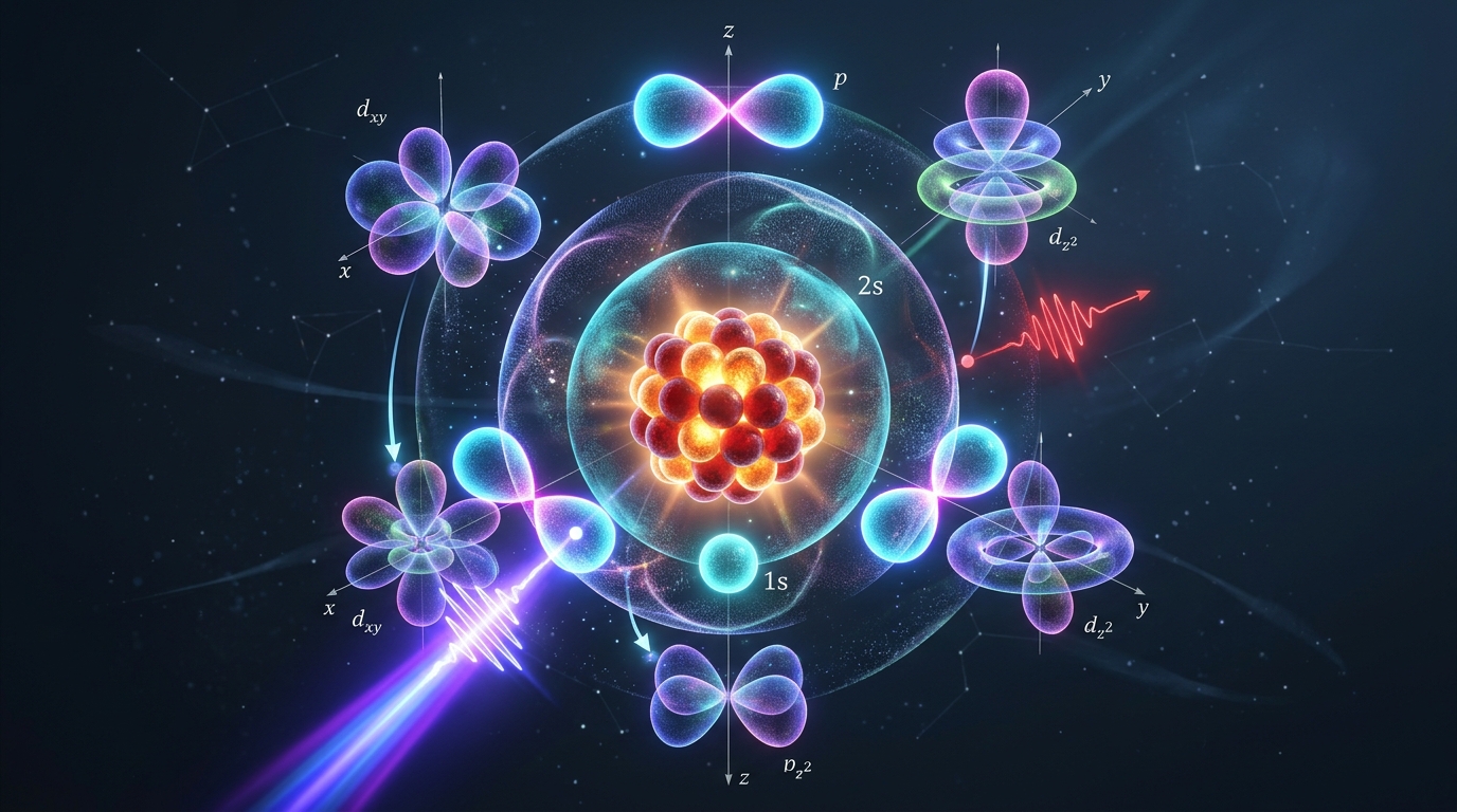
Ilustração 3D das orbitais atómicas hidrogenoides identificadas diretamente na imagem como 1s, 2s, p, d_xy e d_z2 ao longo dos eixos x, y, z em torno do núcleo atómico

Ponte da Secção · Da Leitura à Prática: Pôr os Quatro Modelos a Trabalhar Section Bridge · From Reading to Practice: Putting the Four Models to Work

Percorremos a caixa 1D, a mola vibracional, o rotor e o átomo de Hidrogénio. Cada modelo respondeu a uma pergunta química real: a cor das cenouras, a posição de um pico no infravermelho, porque é que o oxigénio é um tripleto, e a forma das orbitais. Agora é a sua vez! Os exemplos resolvidos mostram o raciocínio passo a passo; os exercícios interativos dão-lhe diagnóstico imediato dos erros mais comuns (fatores esquecidos, sinais trocados, nós mal contados). We have walked through the 1D box, the vibrational spring, the rotor, and the Hydrogen atom. Each model answered a real chemical question: the color of carrots, the position of an infrared peak, why oxygen is a triplet, and the shape of orbitals. Now it is your turn! The worked examples show the reasoning step by step; the interactive exercises give instant diagnostics for the most common mistakes (forgotten factors, swapped signs, miscounted nodes).

9.1 Dois Exemplos Resolvidos Passo a Passo 9.1 Two Step-by-Step Worked Examples

Exemplo Resolvido 5.1 (Partícula na Caixa para o 1,3,5-Hexatrieno Conjugado, $N_\pi = 6$):Worked Example 5.1 (Particle in a Box for Conjugated 1,3,5-Hexatriene, $N_\pi = 6$):
O 1,3,5-hexatrieno tem $3$ ligações duplas conjugadas ($N_\pi = 6$ eletrões $\pi$) numa caixa efetiva de comprimento $L = 7.30\text{ Å}$. Qual é o número quântico do HOMO e do LUMO, quantos nós internos tem cada um e qual é a energia $\Delta E_{\text{HOMO}\to\text{LUMO}}$?
• Ocupação de Pauli: Com $6$ eletrões $\pi$ ($2$ por orbital), o HOMO é $n_{\text{HOMO}} = 6/2 = 3$ ($3 - 1 = \mathbf{2\text{ nós internos}}$) e o LUMO é $n_{\text{LUMO}} = 4$ ($4 - 1 = \mathbf{3\text{ nós internos}}$).
• Energia de transição: Como $\frac{h^2}{8 m_e} = 37.606\text{ eV}\cdot\text{ Å}^2$, temos $\Delta E = \frac{37.606}{(7.30)^2}(4^2 - 3^2) = 0.7057 \times 7 = \mathbf{4.94\text{ eV}}$ ($\lambda = \frac{1239.8}{4.94} = \mathbf{251\text{ nm}}$, valor experimental $= 258\text{ nm}$!). 1,3,5-Hexatriene has $3$ conjugated double bonds ($N_\pi = 6$ $\pi$-electrons) in an effective box of length $L = 7.30\text{ Å}$. What are the HOMO and LUMO quantum numbers, how many internal nodes does each have, and what is $\Delta E_{\text{HOMO}\to\text{LUMO}}$?
• Pauli occupancy: With $6$ $\pi$-electrons ($2$ per orbital), the HOMO is $n_{\text{HOMO}} = 6/2 = 3$ ($3 - 1 = \mathbf{2\text{ internal nodes}}$) and the LUMO is $n_{\text{LUMO}} = 4$ ($4 - 1 = \mathbf{3\text{ internal nodes}}$).
• Transition energy: Using $\frac{h^2}{8 m_e} = 37.606\text{ eV}\cdot\text{ Å}^2$, $\Delta E = \frac{37.606}{(7.30)^2}(4^2 - 3^2) = 0.7057 \times 7 = \mathbf{4.94\text{ eV}}$ ($\lambda = \frac{1239.8}{4.94} = \mathbf{251\text{ nm}}$, experimental value $= 258\text{ nm}$!).

Exemplo Resolvido 8.1 (Análise Completa da Orbital $\text{3p}$ do Átomo de Hidrogénio):Worked Example 8.1 (Complete Analysis of the $\text{3p}$ Orbital of the Hydrogen Atom):
Para uma orbital $\text{3p}$ no átomo de Hidrogénio ($Z = 1$), indique $n, \ell$, nós radiais, nós angulares, nós totais, energia $E_3$ em $\text{E}_\text{h}$ e raio médio $\langle r \rangle_{3p} = \frac{a_0}{2Z}[3n^2 - \ell(\ell+1)]$:
• Números quânticos e nós: $n = 3, \ell = 1 \implies$ Nós radiais $= n - \ell - 1 = 3 - 1 - 1 = \mathbf{1}$; Nós angulares $= \ell = \mathbf{1}$; Nós totais $= n - 1 = \mathbf{2}$.
• Energia e Raio médio: $E_3 = -\frac{1^2}{2(3^2)} = -\frac{1}{18}\text{ E}_\text{h} = \mathbf{-0.05556\text{ E}_\text{h}}$ ($-1.511\text{ eV}$), e $\langle r \rangle_{3p} = \frac{1}{2}[3(9) - 1(2)]\,a_0 = \mathbf{12.5\,a_0 = 6.61\text{ Å}}$. For a $\text{3p}$ orbital in Hydrogen ($Z = 1$), find $n, \ell$, radial nodes, angular nodes, total nodes, energy $E_3$ in $\text{E}_\text{h}$, and mean radius $\langle r \rangle_{3p} = \frac{a_0}{2Z}[3n^2 - \ell(\ell+1)]$:
• Quantum numbers and nodes: $n = 3, \ell = 1 \implies$ Radial nodes $= n - \ell - 1 = 3 - 1 - 1 = \mathbf{1}$; Angular nodes $= \ell = \mathbf{1}$; Total nodes $= n - 1 = \mathbf{2}$.
• Energy and Mean radius: $E_3 = -\frac{1^2}{2(3^2)} = -\frac{1}{18}\text{ E}_\text{h} = \mathbf{-0.05556\text{ E}_\text{h}}$ ($-1.511\text{ eV}$), and $\langle r \rangle_{3p} = \frac{1}{2}[3(9) - 1(2)]\,a_0 = \mathbf{12.5\,a_0 = 6.61\text{ Å}}$.

🎯 Questionário Integrador do Bloco 2 (Autoavaliação e Guia de Estudo)Block 2 Integrative Questionnaire (Self-Assessment & Study Guide)

Reveja os conceitos fundamentais de todos os capítulos deste bloco com diagnóstico automático do que deve estudar mais.Review the fundamental concepts across all chapters of this block with automated diagnostics on what to study further.

0 / 8 (0%)

Modelos Quânticos Analíticos para Química Analytical Quantum Models for Chemistry

A Partícula na Caixa 1D e o Efeito de Túnel The 1D Particle in a Box & Quantum Tunnelling

5.1 Da Corda de Guitarra à Caixa Quântica: Como o Confinamento Cria Quantização 5.1 From Guitar String to Quantum Box: How Confinement Creates Quantization

5.2 A Química da Cor: Porque é que as Cenouras são Laranja e os Tomates Vermelhos? 5.2 The Chemistry of Color: Why Are Carrots Orange and Tomatoes Red?

5.3 Quando as Paredes Não São Infinitas: O Efeito de Túnel Quântico e a Enzima SLO-1 5.3 When Walls Are Not Infinite: Quantum Tunnelling & the SLO-1 Enzyme

Caixa Quântica 1D (Polienos Conjugados) vs. Efeito de Túnel através de Barreira 1D Quantum Box (Conjugated Polyenes) vs. Barrier Tunnelling

📘 Conceito Principal Explicado: Equação de Schrödinger, Interpretação de Born e Aproximação de Born–OppenheimerCore Concept Explained: The Schrödinger Equation, Born Interpretation, and Born–Oppenheimer Approximation

Erwin Schrödinger (1887–1961) ↗

Werner Heisenberg (1901–1976) ↗

Max Born & J. R. Oppenheimer ↗

Wolfgang Pauli & Paul Dirac ↗

Vibrações Moleculares: Do Oscilador Harmónico à Curva de Morse e ao KIE Molecular Vibrations: From the Harmonic Oscillator to the Morse Curve & KIE

6.1 Ligações Químicas como Molas: Massa Reduzida (\(\mu\)), Constante de Força (\(k\)) e Infravermelho 6.1 Chemical Bonds as Springs: Reduced Mass (\(\mu\)), Force Constant (\(k\)) & Infrared Spectroscopy

6.2 A Escada Equidistante do Oscilador Quântico, Regras de Seleção IV e ZPVE 6.2 The Equally Spaced Quantum Oscillator Ladder, IR Selection Rules & ZPVE

6.3 Molas Reais Partem-se! O Potencial Anarmónico de Morse e a Dissociação (\(D_e\) vs. \(D_0\)) 6.3 Real Springs Snap! The Anharmonic Morse Potential & Bond Dissociation (\(D_e\) vs. \(D_0\))

6.4 O Efeito Isotópico Cinético Primário (KIE): Porque é que \(\text{D}_2\text{O}\) e Fármacos Deuterados Reagem Mais Devagar? 6.4 The Primary Kinetic Isotope Effect (KIE): Why Do \(\text{D}_2\text{O}\) & Deuterated Drugs React Slower?

Poço Harmónico vs. Curva de Morse, ZPVE e Calculadora de Efeito Isotópico Cinético (\(k_{\text{H}}/k_{\text{D}}\)) Harmonic Well vs. Morse Curve, ZPVE & Kinetic Isotope Effect (\(k_{\text{H}}/k_{\text{D}}\)) Calculator

Rotação Molecular (Rotor Rígido), Momento Angular Quântico e Spin Molecular Rotation (Rigid Rotor), Quantum Angular Momentum & Spin

7.1 Patinadores no Gelo, Momento de Inércia (\(I = \mu R_e^2\)) e Espectroscopia de Micro-ondas 7.1 Ice Skaters, Moment of Inertia (\(I = \mu R_e^2\)) & Microwave Spectroscopy

7.2 Harmónicas Esféricas \(Y_\ell^{m_\ell}(\theta, \phi)\) e o Cone de Incerteza do Momento Angular 7.2 Spherical Harmonics \(Y_\ell^{m_\ell}(\theta, \phi)\) & the Angular Momentum Uncertainty Cone

7.3 O Mistério de Stern–Gerlach: O Spin Eletrónico (\(s = 1/2\)) e as Matrizes de Pauli 7.3 The Stern–Gerlach Mystery: Electron Spin (\(s = 1/2\)) & the Pauli Matrices

7.4 Multiplicidade de Spin (\(M = 2S+1\)), o Oxigénio Tripleto (\(^3\text{O}_2\)) e o Diagnóstico \(\langle\hat{S}^2\rangle\) no ORCA 7.4 Spin Multiplicity (\(M = 2S+1\)), Triplet Oxygen (\(^3\text{O}_2\)) & the \(\langle\hat{S}^2\rangle\) Diagnostic in ORCA

Escada Rotacional de Micro-ondas (\(E_J\)), Cone de Momento Angular e Auditor de Spin \(\langle\hat{S}^2\rangle\) Microwave Rotational Ladder (\(E_J\)), Angular Momentum Cone & \(\langle\hat{S}^2\rangle\) Spin Auditor

O Átomo de Hidrogénio: Orbitais Atómicas, Cascas de Cebola e Penetração Radial The Hydrogen Atom: Atomic Orbitals, Onion Shells & Radial Penetration

8.1 Fatorização Radial–Angular \(\psi_{n\ell m_\ell}(r,\theta,\phi) = R_{n\ell}(r)\,Y_\ell^{m_\ell}(\theta,\phi)\) e Energias \(E_n\) 8.1 Radial–Angular Factorization \(\psi_{n\ell m_\ell}(r,\theta,\phi) = R_{n\ell}(r)\,Y_\ell^{m_\ell}(\theta,\phi)\) & Energies \(E_n\)

8.2 Os Três Números Quânticos Espaciais \((n, \ell, m_\ell)\) e a Regra Infalível de Contagem de Nós 8.2 The Three Spatial Quantum Numbers \((n, \ell, m_\ell)\) & the Foolproof Node-Counting Rule

8.3 A Analogia das Cascas de Cebola: Densidade Pontual \(|\psi_{1s}(r)|^2\) vs. Função de Distribuição Radial \(P(r) = 4\pi r^2 |\psi_{1s}(r)|^2\) 8.3 The Onion-Shell Analogy: Point Density \(|\psi_{1s}(r)|^2\) vs. Radial Distribution Function \(P(r) = 4\pi r^2 |\psi_{1s}(r)|^2\)

8.4 Penetração Radial e Blindagem (\(Z_{\text{eff}}\)): Porque é que \(E_{2s} \lt E_{2p}\) Constrói a Tabela Periódica? 8.4 Radial Penetration & Shielding (\(Z_{\text{eff}}\)): Why Does \(E_{2s} \lt E_{2p}\) Build the Periodic Table?

Explorador de Orbitais Hidrogenoides (\(1s\text{ a }3d\)): Distribuição Radial \(P_{n\ell}(r)\), Nós e Penetração Hydrogenic Orbital Explorer (\(1s\text{ to }3d\)): Radial Distribution \(P_{n\ell}(r)\), Nodes & Penetration

Exemplos Resolvidos Passo a Passo, Exercícios Numéricos e Quizz Concetual (Bloco II) Step-by-Step Worked Examples, Numerical Exercises & Conceptual Quiz (Block II)

9.1 Dois Exemplos Resolvidos Passo a Passo 9.1 Two Step-by-Step Worked Examples