Bloco III (Capítulos 9–12) — Livro de Texto Interativo: Métodos de Aproximação e o Problema Molecular

Capítulo 9 — Métodos de Aproximação: O Princípio Variacional, o Método de Rayleigh–Ritz e a Teoria das Perturbações de Rayleigh–Schrödinger Chapter 9 — Approximation Methods: The Variational Principle, the Rayleigh–Ritz Method, and Rayleigh–Schrödinger Perturbation Theory

Como resolver com precisão arbitrária a Equação de Schrödinger de átomos multieletrónicos e moléculas quando nenhuma solução analítica fechada existe. How to solve the Schrödinger Equation for multi-electron atoms and molecules to arbitrary accuracy when no closed-form analytical solution exists.

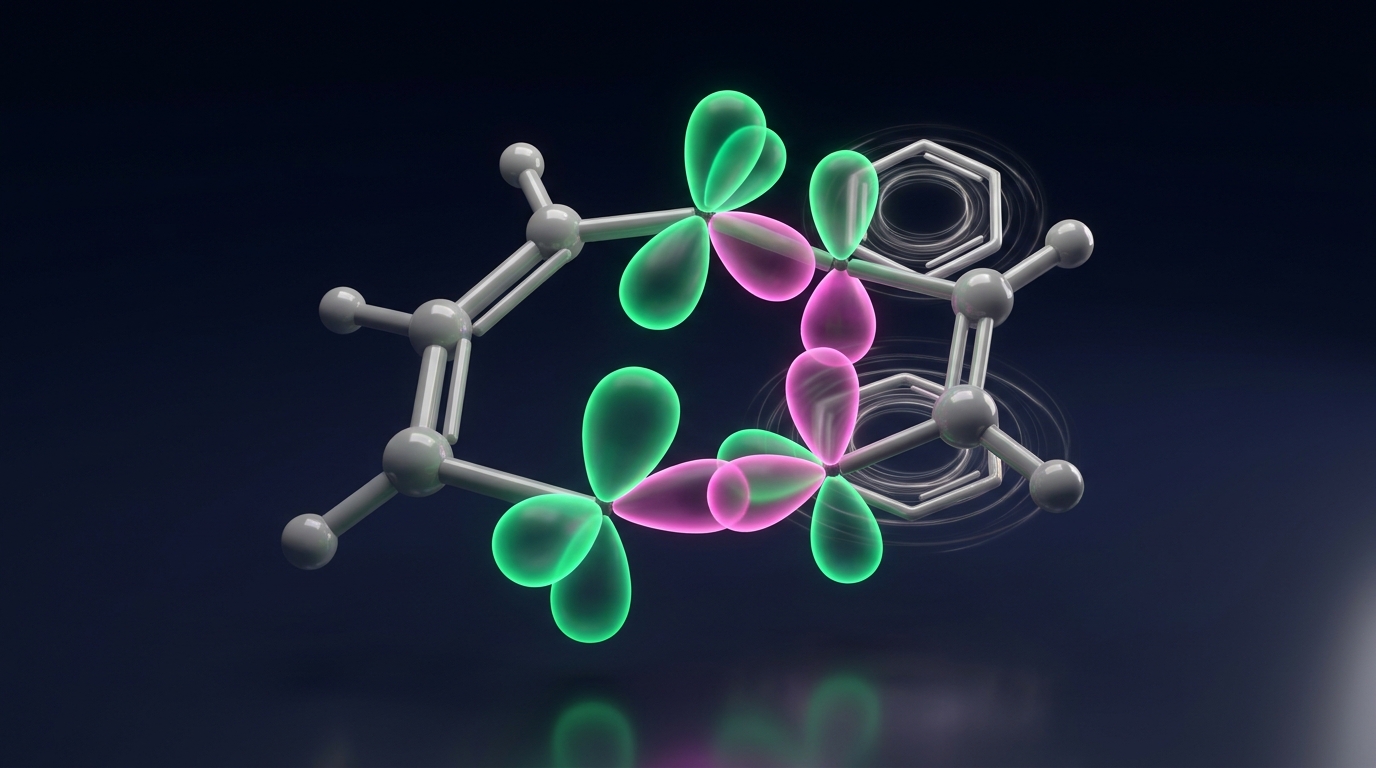
Ilustração 3D da sobreposição de orbitais moleculares de fronteira com lóbulos em verde-esmeralda e magenta sobre um esqueleto conjugado e anéis de deslocalização aromática pi

🌍 Ponto de Partida Químico e Ligação: Porque Precisamos Deste Capítulo?Chemical Starting Point & Connection: Why Do We Need This Chapter?

No final do Bloco II (Capítulo 8), celebrámos um grande triunfo: resolvemos a Equação de Schrödinger exatamente, sem qualquer aproximação, para o átomo de Hidrogénio. De lá saíram as orbitais familiares $1s, 2s, 2p, 3d$ que desenhamos em todas as aulas de Química Geral e Orgânica. Mas há um segredo que os livros introdutórios raramente confessam: o átomo de Hidrogénio (e iões de um só eletrão como o $\text{He}^+$) é o único átomo de toda a Tabela Periódica que pode ser resolvido exatamente com papel e lápis! At the end of Block II (Chapter 8), we celebrated a major triumph: solving the Schrödinger Equation exactly, with zero approximations, for the Hydrogen atom. Out came the familiar $1s, 2s, 2p, 3d$ orbitals we draw in every General and Organic Chemistry class. Yet there is a secret introductory textbooks rarely confess: the Hydrogen atom (and one-electron ions like $\text{He}^+$) is the only atom in the entire Periodic Table that can be solved exactly with pen and paper!

Assim que passamos ao átomo de Hélio (apenas dois eletrões!), à molécula de água, à cafeína ou a uma enzima, os eletrões não só são atraídos pelos núcleos como também se repelem mutuamente a cada instante. Como o movimento de cada eletrão depende instantaneamente de onde estão todos os outros, a matemática exata bloqueia. Significa isto que a Mecânica Quântica é inútil para a Química real? Muito pelo contrário! Neste capítulo vamos descobrir as duas bússolas matemáticas — o Princípio Variacional e a Teoria das Perturbações — que permitem aos químicos computacionais contornar essa barreira e calcular energias de ligação, barreiras de reação e espetros com uma precisão que rivaliza com o melhor laboratório experimental. The moment we move to the Helium atom (just two electrons!), a water molecule, caffeine, or an enzyme, the electrons are not only attracted to the nuclei but also repel one another at every instant. Because each electron's motion depends instantaneously on where every other electron is, exact analytical math hits a wall. Does this mean Quantum Mechanics is useless for real Chemistry? Quite the opposite! In this chapter we will discover the two mathematical compasses — the Variational Principle and Perturbation Theory — that allow computational chemists to bypass this barrier and compute bond energies, reaction barriers, and spectra with an accuracy rivaling the finest experimental laboratory.

9.1 Porque Precisamos de Métodos de Aproximação? A Barreira de $\frac{1}{r_{12}}$ 9.1 Why Do We Need Approximation Methods? The $\frac{1}{r_{12}}$ Barrier

Imagine que está a tentar prever a órbita da Terra em torno do Sol. Se só existirem o Sol e a Terra (um problema de dois corpos), a equação de Newton resolve-se numa linha e dá uma elipse perfeita. Mas se juntar um terceiro corpo fortemente interativo (por exemplo, a Lua ou Júpiter muito próximo), cada puxão gravitacional altera a trajetória dos outros dois em tempo real: é o famoso Problema dos Três Corpos, que não tem fórmula analítica fechada. Imagine trying to predict Earth's orbit around the Sun. If only the Sun and Earth exist (a two-body problem), Newton's equation can be solved in one line and yields a perfect ellipse. But if you add a strongly interacting third body (say, the Moon or a nearby Jupiter), every gravitational tug alters the trajectory of the other two in real time: this is the famous Three-Body Problem, which has no closed-form analytical formula.

Na Química acontece exatamente o mesmo drama logo no segundo elemento da Tabela Periódica. Enquanto num sistema de um único eletrão ($\text{H}$, $\text{He}^+$, $\text{Li}^{2+}$) existe apenas a atração entre o núcleo e o eletrão, assim que adicionamos um segundo eletrão — formando o átomo de Hélio ($\text{He}$, $Z = 2, N = 2$) ou a molécula de hidrogénio ($\text{H}_2$) — surge no Hamiltoniano o operador de repulsão intereletrónica de Coulomb: In Chemistry, the exact same drama unfolds right at the second element of the Periodic Table. Whereas in a one-electron system ($\text{H}$, $\text{He}^+$, $\text{Li}^{2+}$) there is only the attraction between the nucleus and the single electron, the moment we add a second electron — forming the Helium atom ($\text{He}$, $Z = 2, N = 2$) or the hydrogen molecule ($\text{H}_2$) — the interelectronic Coulomb repulsion operator enters the Hamiltonian:

O OPERADOR DE REPULSÃO INTERELETRÓNICA QUE IMPEDE A SEPARAÇÃO DE VARIÁVEISTHE INTERELECTRONIC REPULSION OPERATOR THAT PREVENTS SEPARATION OF VARIABLES $$\hat{V}_{ee}(\mathbf{r}_1, \mathbf{r}_2) = \frac{1}{r_{12}} = \frac{1}{|\mathbf{r}_1 - \mathbf{r}_2|} = \frac{1}{\sqrt{(x_1 - x_2)^2 + (y_1 - y_2)^2 + (z_1 - z_2)^2}}$$

🗣️ O que esta equação significa sem matemática:What this equation means without math: A energia de repulsão entre dois eletrões é inversamente proporcional à distância $r_{12}$ que os separa. Como essa distância mistura as coordenadas $(x_1, y_1, z_1)$ do eletrão 1 com as coordenadas $(x_2, y_2, z_2)$ do eletrão 2 dentro da mesma raiz quadrada no denominador, é matematicamente impossível separar a equação de um átomo multieletrónico em equações independentes para cada eletrão isolado! The repulsion energy between two electrons is inversely proportional to the distance $r_{12}$ separating them. Because that distance mixes the coordinates $(x_1, y_1, z_1)$ of electron 1 with the coordinates $(x_2, y_2, z_2)$ of electron 2 inside the same square root in the denominator, it is mathematically impossible to separate a multi-electron atom's equation into independent equations for each individual electron!

Para vencer esta barreira de $\frac{1}{r_{12}}$, a Química Quântica apoia-se em duas estratégias complementares que sustentam todos os programas modernos como o ORCA, Gaussian ou Q-Chem: To overcome this $\frac{1}{r_{12}}$ barrier, Quantum Chemistry relies on two complementary strategies that underpin every modern software package such as ORCA, Gaussian, or Q-Chem:

O Princípio Variacional (e o Método de Rayleigh–Ritz):The Variational Principle (and the Rayleigh–Ritz Method): Construímos um "molde" flexível de função de onda $\tilde{\Phi}(\mathbf{r}; \alpha_1, \alpha_2, \dots)$ com botões de afinação (parâmetros ajustáveis) e minimizamos o valor esperado da energia $E[\tilde{\Phi}]$. O teorema garante que nunca poderemos descer abaixo da energia verdadeira do estado fundamental $E_0$! We build a flexible wavefunction "mold" $\tilde{\Phi}(\mathbf{r}; \alpha_1, \alpha_2, \dots)$ with tuning knobs (adjustable parameters) and minimize the expectation value of the energy $E[\tilde{\Phi}]$. The theorem guarantees that we can never go below the true ground-state energy $E_0$!
A Teoria das Perturbações de Rayleigh–Schrödinger (RSPT):Rayleigh–Schrödinger Perturbation Theory (RSPT): Partimos de um problema simplificado que sabemos resolver exatamente ($\hat{H}_0$) e adicionamos a diferença para a realidade ($\lambda\hat{V}$) sob a forma de correções sucessivas cada vez mais finas ($E = E^{(0)} + \lambda E^{(1)} + \lambda^2 E^{(2)} + \dots$). We start from a simplified problem we know how to solve exactly ($\hat{H}_0$) and add the difference from reality ($\lambda\hat{V}$) as successive, increasingly refined corrections ($E = E^{(0)} + \lambda E^{(1)} + \lambda^2 E^{(2)} + \dots$).

9.2 O Teorema Variacional: A Bússola Infalível da Química Computacional 9.2 The Variational Theorem: The Infallible Compass of Computational Chemistry

Imagine que procura a altitude do ponto mais fundo de um vale alpino coberto por um nevoeiro cerrado. Mesmo sem conseguir ver o fundo do vale, se caminhar pela montanha com um altímetro no pulso, sabe uma verdade absoluta: qualquer ponto onde ponha os pés terá sempre uma altitude maior ou igual à do fundo verdadeiro do vale. Se der um passo e o altímetro descer, tem a certeza absoluta de que se aproximou da altitude mínima real! Imagine searching for the elevation of the deepest point in an Alpine valley covered in thick fog. Even without seeing the valley floor, if you walk around the mountain with an altimeter on your wrist, you know one absolute truth: any spot where you set foot will always have an elevation greater than or equal to the true valley floor. If you take a step and your altimeter reading drops, you are 100% certain you have moved closer to the true minimum elevation!

Em Mecânica Quântica, a energia exata do estado fundamental $E_0$ é o fundo desse vale, e o valor esperado da energia $E[\tilde{\Phi}]$ de qualquer função de onda de tentativa $\tilde{\Phi}$ funciona como o nosso altímetro. Seja $\hat{H}$ o Hamiltoniano exato de uma molécula, cujas funções próprias exatas ortonormalizadas $\{\Psi_n\}$ e energias exatas ordenadas $E_0 \le E_1 \le E_2 \le \dots$ satisfazem $\hat{H}\Psi_n = E_n\Psi_n$. O Teorema Variacional garante que, para qualquer função de tentativa bem comportada $\tilde{\Phi}$: In Quantum Mechanics, the exact ground-state energy $E_0$ is the floor of that valley, and the energy expectation value $E[\tilde{\Phi}]$ of any trial wavefunction $\tilde{\Phi}$ acts as our altimeter. Let $\hat{H}$ be the exact Hamiltonian of a molecule, whose exact orthonormal eigenfunctions $\{\Psi_n\}$ and ordered exact energies $E_0 \le E_1 \le E_2 \le \dots$ satisfy $\hat{H}\Psi_n = E_n\Psi_n$. The Variational Theorem guarantees that for any well-behaved trial function $\tilde{\Phi}$:

TEOREMA VARIACIONAL (PRINCÍPIO DE RAYLEIGH–RITZ)VARIATIONAL THEOREM (RAYLEIGH–RITZ PRINCIPLE)

$$\begin{gathered} E[\tilde{\Phi}] \equiv \frac{\langle \tilde{\Phi} | \hat{H} | \tilde{\Phi} \rangle}{\langle \tilde{\Phi} | \tilde{\Phi} \rangle} \ge E_0 \\[6pt] \left(\text{com igualdade } E[\tilde{\Phi}] = E_0 \iff \tilde{\Phi} = \Psi_0\right) \end{gathered}$$

$$\begin{gathered} E[\tilde{\Phi}] \equiv \frac{\langle \tilde{\Phi} | \hat{H} | \tilde{\Phi} \rangle}{\langle \tilde{\Phi} | \tilde{\Phi} \rangle} \ge E_0 \\[6pt] \left(\text{with equality } E[\tilde{\Phi}] = E_0 \iff \tilde{\Phi} = \Psi_0\right) \end{gathered}$$

🗣️ O que esta equação significa sem matemática:What this equation means without math: Se inventar qualquer função de onda de tentativa $\tilde{\Phi}$ para descrever os eletrões de uma molécula e calcular a sua energia média $E[\tilde{\Phi}]$, o resultado será sempre superior ou igual à energia verdadeira do estado fundamental $E_0$. Só atingirá exatamente $E_0$ quando a sua função de tentativa coincidir com a função de onda exata da natureza $\Psi_0$. Logo, num cálculo variacional, energia mais baixa (mais negativa) significa sempre uma descrição física mais fiel! If you invent any trial wavefunction $\tilde{\Phi}$ to describe the electrons of a molecule and calculate its average energy $E[\tilde{\Phi}]$, the result will always be greater than or equal to the true ground-state energy $E_0$. You will only hit $E_0$ exactly when your trial function matches nature's exact wavefunction $\Psi_0$. Therefore, in a variational calculation, a lower (more negative) energy always means a more faithful physical description!

💡 Analogia do Quotidiano — O Preço Mínimo Garantido e o Molde de Barro:Everyday Analogy — The Guaranteed Floor Price & The Sculptor's Clay Mold: Porque é que qualquer tentativa imperfeita $\tilde{\Phi}$ dá uma energia acima de $E_0$? Porque no espaço de Hilbert qualquer função imperfeita é, sem darmos por isso, uma mistura do estado fundamental $\Psi_0$ (o mais barato possível, de preço $E_0$) com pequenas contaminações de estados excitados $\Psi_1, \Psi_2, \dots$ (todos mais caros, de preços $E_1, E_2 > E_0$). Se misturar num cesto de compras 95% do produto mais barato da loja com 5% de produtos mais caros, o preço médio por quilo no seu cesto será obrigatoriamente superior ao preço do produto mais barato! Minimizar a energia variacional equivale a limpar a função de onda das contaminações de estados excitados. Why does every imperfect trial function $\tilde{\Phi}$ give an energy above $E_0$? Because in Hilbert space any imperfect function is, behind the scenes, a mixture of the ground state $\Psi_0$ (the cheapest item in the store, priced at $E_0$) with small contaminations of excited states $\Psi_1, \Psi_2, \dots$ (all more expensive, priced at $E_1, E_2 > E_0$). If you fill a shopping basket with 95% of the cheapest item in the store and 5% of more expensive items, the average price per kilogram in your basket is guaranteed to be higher than the cheapest item's price! Minimizing the variational energy is simply purging excited-state contaminations from your trial wavefunction.

📐 Demonstração Passo a Passo do Teorema Variacional (A Prova do "Cesto de Compras" em 4 Passos)Step-by-Step Proof of the Variational Theorem (The "Shopping Basket" Proof in 4 Steps)

Passo 1: Expansão na Base Completa Como $\hat{H}$ é um operador hermitiano, o conjunto das suas funções próprias exatas $\{\Psi_n\}_{n=0}^\infty$ forma uma base completa do espaço de Hilbert. Isto significa que qualquer função de tentativa $\tilde{\Phi}$ pode ser escrita (mesmo sem conhecermos os coeficientes!) como uma combinação linear das funções próprias exatas: Step 1: Completeness Expansion Because $\hat{H}$ is a Hermitian operator, the set of its exact eigenfunctions $\{\Psi_n\}_{n=0}^\infty$ forms a complete basis of the Hilbert space. This means that any trial function $\tilde{\Phi}$ can be expanded (even without knowing the coefficients!) as a linear combination of the exact eigenfunctions:

$$\tilde{\Phi} = \sum_{n=0}^{\infty} c_n \Psi_n, \qquad \text{onde } c_n = \langle \Psi_n | \tilde{\Phi} \rangle$$

$$\tilde{\Phi} = \sum_{n=0}^{\infty} c_n \Psi_n, \qquad \text{where } c_n = \langle \Psi_n | \tilde{\Phi} \rangle$$

Passo 2: Avaliar o Denominador e o Numerador Pela ortonormalidade $\langle \Psi_m | \Psi_n \rangle = \delta_{mn}$ e pela relação de valores próprios $\hat{H}\Psi_n = E_n\Psi_n$, temos: Step 2: Evaluate the Denominator and Numerator Using orthonormality $\langle \Psi_m | \Psi_n \rangle = \delta_{mn}$ and the eigenvalue relation $\hat{H}\Psi_n = E_n\Psi_n$, we obtain:

$$\langle \tilde{\Phi} | \tilde{\Phi} \rangle = \sum_{m=0}^{\infty}\sum_{n=0}^{\infty} c_m^* c_n \underbrace{\langle \Psi_m | \Psi_n \rangle}_{\delta_{mn}} = \sum_{n=0}^{\infty} |c_n|^2$$ $$\langle \tilde{\Phi} | \hat{H} | \tilde{\Phi} \rangle = \sum_{m=0}^{\infty}\sum_{n=0}^{\infty} c_m^* c_n \langle \Psi_m | \hat{H} | \Psi_n \rangle = \sum_{m=0}^{\infty}\sum_{n=0}^{\infty} c_m^* c_n E_n \delta_{mn} = \sum_{n=0}^{\infty} |c_n|^2 E_n$$

Passo 3: Subtrair a Energia do Estado Fundamental $E_0$ Subtraindo $E_0$ ao funcional de Rayleigh $E[\tilde{\Phi}]$, obtemos: Step 3: Subtract the Ground-State Energy $E_0$ Subtracting $E_0$ from the Rayleigh quotient $E[\tilde{\Phi}]$ yields:

$$E[\tilde{\Phi}] - E_0 = \frac{\sum_{n=0}^{\infty} |c_n|^2 E_n}{\sum_{n=0}^{\infty} |c_n|^2} - E_0 \frac{\sum_{n=0}^{\infty} |c_n|^2}{\sum_{n=0}^{\infty} |c_n|^2} = \frac{\sum_{n=0}^{\infty} |c_n|^2 \left(E_n - E_0\right)}{\sum_{n=0}^{\infty} |c_n|^2}$$

Passo 4: Conclusão da Desigualdade Como os quadrados dos módulos são não-negativos ($|c_n|^2 \ge 0$), o denominador é estritamente positivo ($\sum_n |c_n|^2 > 0$), e por definição $E_0$ é o estado de menor energia ($E_n - E_0 \ge 0$ para todo $n$), todas as parcelas da soma são $\ge 0$! Logo: Step 4: Conclude the Inequality Because squared moduli are non-negative ($|c_n|^2 \ge 0$), the denominator is strictly positive ($\sum_n |c_n|^2 > 0$), and by definition $E_0$ is the lowest energy state ($E_n - E_0 \ge 0$ for all $n$), every single term in the sum is $\ge 0$! Therefore:

$$E[\tilde{\Phi}] - E_0 = \frac{\sum_{n=1}^{\infty} |c_n|^2 (E_n - E_0)}{\sum_{n=0}^{\infty} |c_n|^2} \ge 0 \implies E[\tilde{\Phi}] \ge E_0 \qquad \blacksquare$$

💬 Dúvida de Estudante: «Porque é que este teorema é tão poderoso na prática? Significa que na Química Quântica "quanto mais baixa (mais negativa) for a energia, melhor é a função de onda"?»Student Question: "Why is this theorem so powerful in practice? Does it mean that in Quantum Chemistry 'the lower (more negative) the energy, the better the wavefunction'?" Sim — mas APENAS para métodos variacionais! Repare: se a nossa função de tentativa tiver um erro de $1\text{ª}$ ordem relativamente à função exata ($\tilde{\Phi} = \Psi_0 + \delta\Psi$, onde $\|\delta\Psi\| \sim \mathcal{O}(\epsilon)$), a fórmula do Passo 4 mostra que o erro na energia depende de $|c_n|^2 \sim \mathcal{O}(\epsilon^2)$, isto é, o erro na energia é de $2\text{ª}$ ordem (quadrático)! Se a sua função de onda tiver $1\%$ de erro ($0.01$), a sua energia terá um erro da ordem de $(0.01)^2 = 0.01\%$!
Contudo, atenção à distinção fundamental entre métodos de estrutura eletrónica:
• Métodos Variacionais (dão sempre $E_{\text{calc}} \ge E_{\text{exato}}$ na base escolhida): Hartree–Fock ($\text{RHF}, \text{UHF}$), Interação de Configurações ($\text{CISD}, \text{FCI}$) e $\text{CASSCF}$.
• Métodos NÃO-Variacionais (podem dar $E_{\text{calc}} \lt E_{\text{exato}}$): Teoria das Perturbações ($\text{MP2}, \text{CASPT2}$), Coupled Cluster ($\text{CCSD}, \text{CCSD(T)}$) e $\text{DFT}$ de Kohn–Sham aproximada (porque o funcional $E_{\text{XC}}^{\text{aprox}}[\rho]$ é aproximado!). Yes — but ONLY for variational methods! Notice that if our trial wavefunction has a $1\text{st}$-order error relative to the exact wavefunction ($\tilde{\Phi} = \Psi_0 + \delta\Psi$, where $\|\delta\Psi\| \sim \mathcal{O}(\epsilon)$), the formula in Step 4 shows that the energy error depends on $|c_n|^2 \sim \mathcal{O}(\epsilon^2)$ — that is, the energy error is $2\text{nd}$-order (quadratic)! If your wavefunction has a $1\%$ error ($0.01$), your energy error will be on the order of $(0.01)^2 = 0.01\%$!
However, keep in mind the critical distinction across electronic-structure methods:
• Variational Methods (always yield $E_{\text{calc}} \ge E_{\text{exact}}$ within the basis): Hartree–Fock ($\text{RHF}, \text{UHF}$), Configuration Interaction ($\text{CISD}, \text{FCI}$), and $\text{CASSCF}$.
• NON-Variational Methods (can yield $E_{\text{calc}} \lt E_{\text{exact}}$): Perturbation Theory ($\text{MP2}, \text{CASPT2}$), Coupled Cluster ($\text{CCSD}, \text{CCSD(T)}$), and approximate Kohn–Sham $\text{DFT}$ (because the functional $E_{\text{XC}}^{\text{approx}}[\rho]$ is approximate!).

9.3 O Método Linear de Rayleigh–Ritz: De Equações Diferenciais a Matrizes no Computador 9.3 The Linear Rayleigh–Ritz Method: Turning Differential Equations into Computer Matrices

Os computadores digitais não sabem "adivinhar funções" abstratas, mas são extraordinariamente rápidos a multiplicar matrizes e resolver sistemas de equações lineares. Como transformar então a procura variacional da melhor função de onda num problema de matrizes? Digital computers do not know how to "guess abstract functions", but they are extraordinarily fast at multiplying matrices and solving systems of linear equations. How, then, can we turn the variational search for the best wavefunction into a matrix problem?

Walther Ritz (1909) e Lord Rayleigh propuseram a ideia genial que hoje usamos em todos os cálculos de orbitais moleculares (LCAO): escolhemos um conjunto finito de $M$ funções de base conhecidas $\{\phi_1, \phi_2, \dots, \phi_M\}$ — como os blocos de construção atómicos centrados em cada núcleo — e escrevemos a função de tentativa $\tilde{\Phi}$ como uma combinação linear dessas funções, onde os únicos parâmetros a otimizar são os pesos numéricos (coeficientes) $c_1, c_2, \dots, c_M$: Walther Ritz (1909) and Lord Rayleigh proposed the brilliant idea we use today in every molecular orbital (LCAO) calculation: we pick a finite set of $M$ known basis functions $\{\phi_1, \phi_2, \dots, \phi_M\}$ — like atomic building blocks centered on each nucleus — and write the trial function $\tilde{\Phi}$ as a linear combination of those functions, where the only parameters to optimize are the numerical weights (coefficients) $c_1, c_2, \dots, c_M$:

EXPANSÃO LINEAR DE RAYLEIGH–RITZ E MATRIZES $\mathbf{H}$ E $\mathbf{S}$RAYLEIGH–RITZ LINEAR EXPANSION & MATRICES $\mathbf{H}$ AND $\mathbf{S}$ $$\begin{gathered} \tilde{\Phi} = \sum_{\nu=1}^{M} c_\nu \phi_\nu \\[6pt] \implies\; E(\mathbf{c}) = \frac{\sum_{\mu=1}^M \sum_{\nu=1}^M c_\mu^* c_\nu H_{\mu\nu}}{\sum_{\mu=1}^M \sum_{\nu=1}^M c_\mu^* c_\nu S_{\mu\nu}} = \frac{\mathbf{c}^\dagger \mathbf{H} \mathbf{c}}{\mathbf{c}^\dagger \mathbf{S} \mathbf{c}} \end{gathered}$$

$$\text{onde}\quad H_{\mu\nu} \equiv \langle \phi_\mu | \hat{H} | \phi_\nu \rangle = \int \phi_\mu^*(\mathbf{r})\hat{H}\phi_\nu(\mathbf{r})\,d\tau \quad\text{e}\quad S_{\mu\nu} \equiv \langle \phi_\mu | \phi_\nu \rangle = \int \phi_\mu^*(\mathbf{r})\phi_\nu(\mathbf{r})\,d\tau$$

$$\text{where}\quad H_{\mu\nu} \equiv \langle \phi_\mu | \hat{H} | \phi_\nu \rangle = \int \phi_\mu^*(\mathbf{r})\hat{H}\phi_\nu(\mathbf{r})\,d\tau \quad\text{and}\quad S_{\mu\nu} \equiv \langle \phi_\mu | \phi_\nu \rangle = \int \phi_\mu^*(\mathbf{r})\phi_\nu(\mathbf{r})\,d\tau$$

🗣️ O que esta equação significa sem matemática:What this equation means without math: Em vez de trabalhar com funções contínuas infinitas, guardamos toda a física da molécula em duas tabelas quadradas de números ($M \times M$): a matriz Hamiltoniana $\mathbf{H}$ (onde $H_{\mu\nu}$ mede a energia de interação entre as funções de base $\phi_\mu$ e $\phi_\nu$) e a matriz de sobreposição $\mathbf{S}$ (onde $S_{\mu\nu}$ mede quanto as nuvens $\phi_\mu$ e $\phi_\nu$ se interpenetram no espaço). Instead of working with infinite continuous functions, we store all the physics of the molecule inside two square tables of numbers ($M \times M$): the Hamiltonian matrix $\mathbf{H}$ (where $H_{\mu\nu}$ measures the interaction energy between basis functions $\phi_\mu$ and $\phi_\nu$) and the overlap matrix $\mathbf{S}$ (where $S_{\mu\nu}$ measures how much clouds $\phi_\mu$ and $\phi_\nu$ interpenetrate in space).

Para encontrar os coeficientes ótimos $\{c_\nu\}$ que tornam a energia $E(\mathbf{c})$ mínima, derivamos em ordem a cada coeficiente $c_\mu^*$ e igualamos a derivada a zero ($\frac{\partial E}{\partial c_\mu^*} = 0$ para $\mu = 1, \dots, M$), obtendo as célebres Equações Seculares de Rayleigh–Ritz: To find the optimal coefficients $\{c_\nu\}$ that minimize the energy $E(\mathbf{c})$, we differentiate with respect to each coefficient $c_\mu^*$ and set the derivative to zero ($\frac{\partial E}{\partial c_\mu^*} = 0$ for $\mu = 1, \dots, M$), obtaining the famous Rayleigh–Ritz Secular Equations:

EQUAÇÕES SECULARES DE RAYLEIGH–RITZ E DETERMINANTE SECULARRAYLEIGH–RITZ SECULAR EQUATIONS & SECULAR DETERMINANT $$\begin{gathered} \sum_{\nu=1}^{M} \left(H_{\mu\nu} - E\,S_{\mu\nu}\right) c_\nu = 0 \quad (\mu = 1, \dots, M) \; \\[6pt] \Longleftrightarrow\; \; \mathbf{H}\mathbf{c} = E\mathbf{S}\mathbf{c} \; \\[6pt] \Longleftrightarrow\; \; \det\!\left(\mathbf{H} - E\mathbf{S}\right) = 0 \end{gathered}$$

🗣️ O que esta equação significa sem matemática:What this equation means without math: Se usar $M$ orbitais atómicas para construir uma molécula, o determinante secular $\det(\mathbf{H} - E\mathbf{S}) = 0$ dá-lhe exatamente $M$ níveis de energia permitidos ($\tilde{E}_0 \le \tilde{E}_1 \le \dots \le \tilde{E}_{M-1}$) — ou seja, de $M$ orbitais atómicas nascem exatamente $M$ orbitais moleculares! Além disso, se aumentar o número de funções de base ($M \to M+1$), todas as energias calculadas descem (ou mantêm-se), aproximando-se cada vez mais das energias exatas da natureza. If you use $M$ atomic orbitals to build a molecule, the secular determinant $\det(\mathbf{H} - E\mathbf{S}) = 0$ gives you exactly $M$ allowed energy levels ($\tilde{E}_0 \le \tilde{E}_1 \le \dots \le \tilde{E}_{M-1}$) — in other words, $M$ atomic orbitals always produce exactly $M$ molecular orbitals! Furthermore, if you add more basis functions ($M \to M+1$), every computed energy level drops (or stays the same), approaching nature's exact energies ever more closely.

9.4 Teoria das Perturbações de Rayleigh–Schrödinger (RSPT) 9.4 Rayleigh–Schrödinger Perturbation Theory (RSPT)

Imagine que quer calcular o seu rendimento líquido anual depois de o governo anunciar um pequeno bónus fiscal, ou que os astrónomos do século XIX queriam calcular a órbita da Terra (dominada a $99.9\%$ pela gravidade do Sol) incluindo o pequeno puxão gravitacional extra de Júpiter. Ninguém deita fora a órbita elíptica em torno do Sol para começar do zero! Em vez disso, toma-se a solução simples conhecida (ordem zero) e calcula-se o pequeno desvio causado pela perturbação. Imagine calculating your net annual salary after a small tax bonus is announced, or 19th-century astronomers computing Earth's orbit (dominated $99.9\%$ by the Sun's gravity) while accounting for the tiny extra gravitational tug of Jupiter. Nobody throws away the elliptical solar orbit to start from scratch! Instead, you take the known simple solution (zeroth order) and compute the small shift caused by the perturbation.

💡 Analogia do Quotidiano — O Salário Base e os Ajustes Sucessivos:Everyday Analogy — Base Salary & Successive Adjustments: A Teoria das Perturbações funciona exatamente como um recibo de vencimento: $E^{(0)}$ é o salário base fixo (fácil de saber de cor); $E^{(1)}$ é o ajuste de $1\text{ª}$ ordem (calcular o bónus olhando apenas para o seu horário habitual, sem mudar a sua rotina); e $E^{(2)}$ é a resposta de $2\text{ª}$ ordem (como o bónus existe, você adapta ligeiramente o seu horário para aproveitar horas extraordinárias, o que baixa ainda mais a energia do sistema!). Perturbation Theory works just like a paycheck: $E^{(0)}$ is your fixed base salary (known by heart); $E^{(1)}$ is the $1\text{st}$-order adjustment (evaluating the bonus using your existing routine without changing your schedule); and $E^{(2)}$ is the $2\text{nd}$-order response (because the bonus exists, you slightly adapt your schedule to capture overtime, which lowers the system's energy even further!).

Matematicamente, quando o Hamiltoniano exato $\hat{H}$ difere apenas por um termo relativamente pequeno $\hat{V}$ de um Hamiltoniano de referência $\hat{H}_0$ cujos estados próprios ortonormalizados $\hat{H}_0 |\psi_n^{(0)}\rangle = E_n^{(0)} |\psi_n^{(0)}\rangle$ já conhecemos exatamente, partimos $\hat{H}$ introduzindo um botão contínuo $\lambda \in [0, 1]$ que "liga" a perturbação: Mathematically, when the exact Hamiltonian $\hat{H}$ differs by a relatively small term $\hat{V}$ from a reference Hamiltonian $\hat{H}_0$ whose orthonormal eigenstates $\hat{H}_0 |\psi_n^{(0)}\rangle = E_n^{(0)} |\psi_n^{(0)}\rangle$ are already known exactly, we partition $\hat{H}$ using a continuous dial $\lambda \in [0, 1]$ that "turns on" the perturbation:

EXPANSÃO EM SÉRIE DE POTÊNCIAS DE RAYLEIGH–SCHRÖDINGERRAYLEIGH–SCHRÖDINGER POWER-SERIES EXPANSION $$\begin{gathered} \hat{H}(\lambda) = \hat{H}_0 + \lambda\hat{V} \\[6pt] E_n(\lambda) = E_n^{(0)} + \lambda E_n^{(1)} + \lambda^2 E_n^{(2)} + \dots \\[6pt] |\Psi_n(\lambda)\rangle = |\psi_n^{(0)}\rangle + \lambda |\psi_n^{(1)}\rangle + \lambda^2 |\psi_n^{(2)}\rangle + \dots \end{gathered}$$

🗣️ O que esta equação significa sem matemática:What this equation means without math: Quando $\lambda = 0$, temos o problema fácil já resolvido; quando $\lambda = 1$, temos a molécula real completa. As correções $E_n^{(1)}, E_n^{(2)}, \dots$ dizem-nos quanto a energia muda em primeira aproximação, segunda aproximação, e assim sucessivamente. When $\lambda = 0$, we have the easy, already-solved problem; when $\lambda = 1$, we have the full real molecule. The corrections $E_n^{(1)}, E_n^{(2)}, \dots$ tell us how much the energy shifts in first approximation, second approximation, and so on.

Substituindo na equação de Schrödinger e agrupando termos com a mesma potência de $\lambda$, surgem as três fórmulas mais famosas da Teoria das Perturbações (que no Capítulo 15 darão origem ao método $\text{MP2}$): Substituting into the Schrödinger equation and grouping terms with the same power of $\lambda$ yields the three most famous formulas of Perturbation Theory (which in Chapter 15 will give rise to the $\text{MP2}$ method):

Ordem $\lambda^1$: Energia $E_n^{(1)}$Order $\lambda^1$: Energy $E_n^{(1)}$

Média da Perturbação na Função de Ordem Zero:Expectation Value of $\hat{V}$ over the Unperturbed State:
$$E_n^{(1)} = \langle \psi_n^{(0)} | \hat{V} | \psi_n^{(0)} \rangle$$ Para calcular a energia até $1\text{ª}$ ordem ($E_n^{(0)} + E_n^{(1)}$), basta conhecer a função de onda de ordem zero $|\psi_n^{(0)}\rangle$! To compute the energy through $1\text{st}$ order ($E_n^{(0)} + E_n^{(1)}$), you only need the zeroth-order wavefunction $|\psi_n^{(0)}\rangle$!

Ordem $\lambda^1$: Estado $|\psi_n^{(1)}\rangle$Order $\lambda^1$: State $|\psi_n^{(1)}\rangle$

Mistura de Estados Excitados pela Perturbação:Mixing of Excited States Induced by $\hat{V}$:
$$|\psi_n^{(1)}\rangle = \sum_{k \neq n} \frac{\langle \psi_k^{(0)} | \hat{V} | \psi_n^{(0)} \rangle}{E_n^{(0)} - E_k^{(0)}} |\psi_k^{(0)}\rangle$$ A perturbação deforma a nuvem eletrónica misturando pequenos contributos de estados excitados $k \neq n$. The perturbation polarizes the electron cloud by mixing in small contributions from excited states $k \neq n$.

Ordem $\lambda^2$: Energia $E_0^{(2)} \le 0$Order $\lambda^2$: Energy $E_0^{(2)} \le 0$

Correção de $2\text{ª}$ Ordem ao Estado Fundamental:$2\text{nd}$-Order Ground-State Energy Correction:
$$E_0^{(2)} = \sum_{k \neq 0} \frac{|\langle \psi_0^{(0)} | \hat{V} | \psi_k^{(0)} \rangle|^2}{E_0^{(0)} - E_k^{(0)}} \le 0$$ Como o numerador é $\ge 0$ e o denominador $E_0^{(0)} - E_k^{(0)} \lt 0$ para o estado fundamental, $E_0^{(2)}$ é sempre negativa (estabilizadora)! Because the numerator is $\ge 0$ and the denominator $E_0^{(0)} - E_k^{(0)} \lt 0$ for the ground state, $E_0^{(2)}$ is always negative (stabilizing)!

🧪 Paralelo Real em Química Computacional — Porque é que as Moléculas Polarizam num Campo Elétrico e Quando é que o MP2 Explode?Real-World Parallel in Computational Chemistry — Why Molecules Polarize in an Electric Field & When Does MP2 Explode? Olhe para a fórmula de $E_0^{(2)}$ acima: porque é que é sempre negativa? Porque quando aplicamos uma perturbação (por exemplo, aproximar um catião $\text{Na}^+$ de uma molécula de benzeno), a nuvem eletrónica do estado fundamental $\psi_0^{(0)}$ deforma-se misturando orbitais excitadas vazias $\psi_k^{(0)}$ para se acomodar à perturbação e baixar a sua energia (é a origem física da polarizabilidade $\alpha$ e das forças de dispersão de London!).
Mas repare no denominador $E_0^{(0)} - E_k^{(0)}$ (o hiato HOMO–LUMO): se esticarmos uma ligação covalente até a quebrar, o nível ligante ($\sigma$) e o antiligante ($\sigma^*$) ficam com a mesma energia ($E_k^{(0)} \to E_0^{(0)}$). Dividir por zero faz com que $E_0^{(2)} \to -\infty$! É por isso que nunca se deve usar teoria das perturbações de referência única ($\text{MP2}$) para estudar quebras homolíticas de ligações ou metais de transição com orbitais $d$ quase degeneradas. Look at the formula for $E_0^{(2)}$ above: why is it always negative? Because when we apply a perturbation (for instance, bringing a $\text{Na}^+$ cation near a benzene ring), the ground-state electron cloud $\psi_0^{(0)}$ deforms by mixing in empty excited orbitals $\psi_k^{(0)}$ to accommodate the perturbation and lower its energy (this is the physical origin of polarizability $\alpha$ and London dispersion forces!).
However, look at the denominator $E_0^{(0)} - E_k^{(0)}$ (the HOMO–LUMO gap): if we stretch a covalent bond to breaking, the bonding ($\sigma$) and antibonding ($\sigma^*$) levels approach the exact same energy ($E_k^{(0)} \to E_0^{(0)}$). Dividing by zero sends $E_0^{(2)} \to -\infty$! That is why single-reference perturbation theory ($\text{MP2}$) must never be used for homolytic bond breaking or transition metals with nearly degenerate $d$ orbitals.

9.5 Exemplo Resolvido e Simulador: O Átomo de Hélio ($\text{He}$, $Z = 2$) e o Efeito de Blindagem Eletrónica 9.5 Worked Example & Simulator: The Helium Atom ($\text{He}$, $Z = 2$) and Electronic Shielding

Em Química Geral aprendemos as Regras de Blindagem de Slater: num átomo com vários eletrões, um eletrão não sente a carga total $Z$ do núcleo porque os outros eletrões fazem uma "cortina" (blindagem ou ecranização, $\sigma$), reduzindo a carga sentida para uma Carga Nuclear Efetiva $Z_{\text{eff}} = Z - \sigma$. Mas de onde vem fisicamente esse número $\sigma$? Vem diretamente do Princípio Variacional! In General Chemistry we learn Slater's Shielding Rules: in a multi-electron atom, an electron does not feel the full nuclear charge $Z$ because the other electrons act as a "curtain" (shielding or screening, $\sigma$), reducing the felt charge to an Effective Nuclear Charge $Z_{\text{eff}} = Z - \sigma$. Where does that shielding number $\sigma$ physically come from? Directly from the Variational Principle!

Apliquemos tanto a Teoria das Perturbações como o Princípio Variacional ao átomo de Hélio ($Z = 2$, dois eletrões na configuração $1s^2$), cujo Hamiltoniano exato em unidades atómicas é $\hat{H} = \left(-\frac{1}{2}\nabla_1^2 - \frac{Z}{r_1}\right) + \left(-\frac{1}{2}\nabla_2^2 - \frac{Z}{r_2}\right) + \frac{1}{r_{12}}$, e cuja energia experimental/exata é $E_{\text{exato}}(\text{He}) = -2.903724\text{ E}_\text{h}$ ($-79.01\text{ eV}$): Let us apply both Perturbation Theory and the Variational Principle to the Helium atom ($Z = 2$, two electrons in the $1s^2$ configuration), whose exact Hamiltonian in atomic units is $\hat{H} = \left(-\frac{1}{2}\nabla_1^2 - \frac{Z}{r_1}\right) + \left(-\frac{1}{2}\nabla_2^2 - \frac{Z}{r_2}\right) + \frac{1}{r_{12}}$, and whose exact energy is $E_{\text{exact}}(\text{He}) = -2.903724\text{ E}_\text{h}$ ($-79.01\text{ eV}$):

1. Aproximação de Ordem Zero (Ignorando a Repulsão $\frac{1}{r_{12}}$):1. Zeroth-Order Approximation (Ignoring $\frac{1}{r_{12}}$ Repulsion):
Se os dois eletrões fossem fantasmas invisíveis um para o outro ($\hat{V} = 0$), cada um sentiria o núcleo nu $Z = 2$ com energia hidrogenoide $-Z^2/2 = -2.0000\text{ E}_\text{h}$: If the two electrons were ghosts invisible to each other ($\hat{V} = 0$), each would feel the bare nucleus $Z = 2$ with hydrogenic energy $-Z^2/2 = -2.0000\text{ E}_\text{h}$:

$$E^{(0)} = -\frac{Z^2}{2} - \frac{Z^2}{2} = -Z^2 = -4.0000\text{ E}_\text{h} \qquad (\text{Erro brutal de }-1.096\text{ E}_\text{h} = -688\text{ kcal/mol!})$$

$$E^{(0)} = -\frac{Z^2}{2} - \frac{Z^2}{2} = -Z^2 = -4.0000\text{ E}_\text{h} \qquad (\text{Massive error of }-1.096\text{ E}_\text{h} = -688\text{ kcal/mol!})$$

2. Teoria das Perturbações de $1\text{ª}$ Ordem ($E^{(0)} + E^{(1)}$):2. First-Order Perturbation Theory ($E^{(0)} + E^{(1)}$):
Mantendo as orbitais $1s$ rígidas com $Z = 2$ ($\psi^{(0)}(r_1,r_2) = \frac{Z^3}{\pi}e^{-Z(r_1+r_2)}$), calculamos a repulsão média $\langle \psi^{(0)} | \frac{1}{r_{12}} | \psi^{(0)} \rangle = \frac{5}{8}Z$: Keeping the $1s$ orbitals rigid with $Z = 2$ ($\psi^{(0)}(r_1,r_2) = \frac{Z^3}{\pi}e^{-Z(r_1+r_2)}$), we evaluate the average repulsion $\langle \psi^{(0)} | \frac{1}{r_{12}} | \psi^{(0)} \rangle = \frac{5}{8}Z$:

$$E^{(0+1)} = -Z^2 + \frac{5}{8}Z = -4 + \frac{10}{8} = \mathbf{-2.7500\text{ E}_\text{h}} \qquad (\text{Erro reduzido para }+0.1537\text{ E}_\text{h} = +96.5\text{ kcal/mol})$$

$$E^{(0+1)} = -Z^2 + \frac{5}{8}Z = -4 + \frac{10}{8} = \mathbf{-2.7500\text{ E}_\text{h}} \qquad (\text{Error reduced to }+0.1537\text{ E}_\text{h} = +96.5\text{ kcal/mol})$$

3. Otimização Variacional da Carga Nuclear Efetiva $\zeta = Z_{\text{eff}}$ (Kellner, 1927):3. Variational Optimization of the Effective Nuclear Charge $\zeta = Z_{\text{eff}}$ (Kellner, 1927):
Fisicamente, como os dois eletrões se repelem, a nuvem eletrónica incha ligeiramente porque cada eletrão blinda parcialmente o núcleo para o outro! Substituindo $Z$ na função de onda por uma carga nuclear efetiva ajustável $\zeta$ ($\tilde{\Phi}(r_1,r_2;\zeta) = \frac{\zeta^3}{\pi}e^{-\zeta(r_1+r_2)}$), a energia variacional em função de $\zeta$ é: Physically, because the two electrons repel each other, the electron cloud swells slightly as each electron partially shields the nucleus from the other! Replacing $Z$ in the wavefunction by an adjustable effective nuclear charge $\zeta$ ($\tilde{\Phi}(r_1,r_2;\zeta) = \frac{\zeta^3}{\pi}e^{-\zeta(r_1+r_2)}$), the variational energy as a function of $\zeta$ is: $$E(\zeta) = \underbrace{\zeta^2}_{\langle \hat{T}_e \rangle} - \underbrace{2Z\zeta}_{-\langle \hat{V}_{ne} \rangle} + \underbrace{\frac{5}{8}\zeta}_{\langle \hat{V}_{ee} \rangle} = \zeta^2 - \left(2Z - \frac{5}{8}\right)\zeta$$ Minimizando em ordem a $\zeta$:Minimizing with respect to $\zeta$:

$$\frac{dE(\zeta)}{d\zeta} = 2\zeta - \left(2Z - \frac{5}{8}\right) = 0 \implies \zeta_{\text{ótimo}} = Z - \frac{5}{16} = 2 - 0.3125 = \mathbf{1.6875}$$ $$\begin{gathered} E_{\text{var}}(\zeta_{\text{ótimo}}) = -\left(Z - \frac{5}{16}\right)^2 = -(1.6875)^2 = \mathbf{-2.847656\text{ E}_\text{h}} \\[6pt] (\text{Acima de } E_{\text{exato}} = -2.903724\text{ E}_\text{h}\text{!}) \end{gathered}$$

$$\frac{dE(\zeta)}{d\zeta} = 2\zeta - \left(2Z - \frac{5}{8}\right) = 0 \implies \zeta_{\text{opt}} = Z - \frac{5}{16} = 2 - 0.3125 = \mathbf{1.6875}$$ $$\begin{gathered} E_{\text{var}}(\zeta_{\text{opt}}) = -\left(Z - \frac{5}{16}\right)^2 = -(1.6875)^2 = \mathbf{-2.847656\text{ E}_\text{h}} \\[6pt] (\text{Above } E_{\text{exact}} = -2.903724\text{ E}_\text{h}\text{!}) \end{gathered}$$

🧪 Conexão Direta com a Tabela Periódica — De Onde Vem a Constante de Blindagem $\sigma = 0.30$ de Slater?Direct Connection to the Periodic Table — Where Does Slater's Shielding Constant $\sigma = 0.30$ Come From? Olhe para o resultado variacional que acabámos de deduzir sem qualquer parâmetro empírico: $\zeta_{\text{ótimo}} = Z - \frac{5}{16} = Z - 0.3125$! Ou seja, um eletrão $1s$ blinda exatamente $\frac{5}{16} = \mathbf{0.3125}$ de unidade de carga nuclear ao seu companheiro de orbital $1s$! Quando John C. Slater propôs em 1930 as suas famosas regras empíricas de blindagem para toda a Tabela Periódica, arredondou este valor exato $0.3125$ para $\sigma_{1s} = 0.30$! Graças a esta blindagem, a 1.ª energia de ionização do Hélio não é $54.4\text{ eV}$ (valor sem repulsão), mas sim $\text{IP}_1(\text{He}) = E(\text{He}^+) - E(\text{He}) = (-2.000) - (-2.9037) = 0.9037\text{ E}_\text{h} = \mathbf{24.59\text{ eV}}$. Look at the variational result we just derived with zero empirical parameters: $\zeta_{\text{opt}} = Z - \frac{5}{16} = Z - 0.3125$! In other words, one $1s$ electron shields exactly $\frac{5}{16} = \mathbf{0.3125}$ of a unit of nuclear charge from its $1s$ orbital partner! When John C. Slater proposed his famous empirical shielding rules for the Periodic Table in 1930, he simply rounded this exact theoretical value $0.3125$ to $\sigma_{1s} = 0.30$! Thanks to this shielding, the 1st ionization energy of Helium is not $54.4\text{ eV}$ (the unshielded value), but $\text{IP}_1(\text{He}) = E(\text{He}^+) - E(\text{He}) = (-2.000) - (-2.9037) = 0.9037\text{ E}_\text{h} = \mathbf{24.59\text{ eV}}$.

💬 Dúvida de Estudante: «Com $\zeta = 1.6875$ chegámos a $-2.8477\text{ E}_\text{h}$, e mesmo o melhor orbital $1s$ numérico (Hartree–Fock, Cap. 13) dá $-2.8617\text{ E}_\text{h}$. Onde estão os restantes $0.0420\text{ E}_\text{h}$ ($26.4\text{ kcal/mol}$) que faltam para a energia exata $-2.9037\text{ E}_\text{h}$?»Student Question: "With $\zeta = 1.6875$ we reached $-2.8477\text{ E}_\text{h}$, and even the best numerical $1s$ orbital (Hartree–Fock, Ch. 13) gives $-2.8617\text{ E}_\text{h}$. Where are the remaining $0.0420\text{ E}_\text{h}$ ($26.4\text{ kcal/mol}$) missing from the exact energy $-2.9037\text{ E}_\text{h}$?" Essa diferença de $-0.0420\text{ E}_\text{h}$ chama-se Energia de Correlação Eletrónica (que estudaremos a fundo no Capítulo 15)! Quando escrevemos $\tilde{\Phi}(r_1, r_2) = \phi_{1s}(r_1)\phi_{1s}(r_2)$, assumimos que a probabilidade de encontrar o eletrão 1 numa posição não depende de onde está o eletrão 2 nesse instante. Na realidade, os dois eletrões evitam-se dinamicamente (quando o eletrão 1 está à esquerda do núcleo, o eletrão 2 prefere estar à direita). Quando Egil Hylleraas (1929) incluiu explicitamente a distância $r_{12}$ na função de onda variacional, a energia desceu imediatamente para $-2.9037\text{ E}_\text{h}$! That missing $-0.0420\text{ E}_\text{h}$ is called the Electron Correlation Energy (which we will study in depth in Chapter 15)! When we write $\tilde{\Phi}(r_1, r_2) = \phi_{1s}(r_1)\phi_{1s}(r_2)$, we assume the probability of finding electron 1 at a given spot does not depend on where electron 2 is at that instant. In reality, the two electrons dynamically avoid each other (when electron 1 is to the left of the nucleus, electron 2 prefers to be on the right). When Egil Hylleraas (1929) explicitly included the interelectronic distance $r_{12}$ in the variational trial wavefunction, the energy immediately dropped to $-2.9037\text{ E}_\text{h}$!

🔬 Interativo 9.1Interactive 9.1 Otimizador Variacional da Carga Nuclear Efetiva $\zeta$ para o Átomo de Hélio ($\text{He}$, $1s^2$) Variational Effective Nuclear Charge $\zeta$ Optimizer for the Helium Atom ($\text{He}$, $1s^2$)

Arraste o cursor do expoente orbital $\zeta$ e veja como o compromisso entre a energia cinética $\langle \hat{T}_e \rangle = \zeta^2$ e a energia potencial $\langle \hat{V} \rangle = -\left(4 - \frac{5}{8}\right)\zeta$ produz uma parábola cujo mínimo ocorre exatamente em $\zeta = \frac{27}{16} = 1.6875$, respeitando sempre $E(\zeta) \ge E_{\text{HF}} = -2.8617\text{ E}_\text{h} > E_{\text{exato}} = -2.9037\text{ E}_\text{h}$: Drag the orbital exponent slider $\zeta$ and watch how the trade-off between kinetic energy $\langle \hat{T}_e \rangle = \zeta^2$ and potential energy $\langle \hat{V} \rangle = -\left(4 - \frac{5}{8}\right)\zeta$ produces a parabola whose minimum lies at $\zeta = \frac{27}{16} = 1.6875$, strictly obeying $E(\zeta) \ge E_{\text{HF}} = -2.8617\text{ E}_\text{h} > E_{\text{exact}} = -2.9037\text{ E}_\text{h}$:

🎯 O Que Se Pretende Fazer Neste Simulador e Porquê What This Simulator Does & Why It Matters

Objetivo: Aplicar o Princípio Variacional ao átomo de Hélio (Capítulo 9). Desloque o expoente $\zeta$ da orbital $1s$ e observe como a competição entre energia cinética, atração nuclear e repulsão eletrónica $J_{11}$ atinge o mínimo exato em $\zeta = 1.6875$, mantendo-se sempre acima da energia exata $-2.9037\text{ E}_\text{h}$. Goal: Apply the Variational Principle to the Helium atom (Chapter 9). Slide the $1s$ orbital exponent $\zeta$ and watch how the competition among kinetic energy, nuclear attraction, and electron repulsion $J_{11}$ reaches its exact minimum at $\zeta = 1.6875$, staying strictly above the exact energy $-2.9037\text{ E}_\text{h}$.

Expoente Variacional $\zeta$ ($a_0^{-1}$):Variational Exponent $\zeta$ ($a_0^{-1}$): 1.6875

ℹ️ Explicação deste seletor / controlo (clique para abrir)ℹ️ Explanation of this selector / control (click to open)

O que controla: Ajusta o expoente orbital variacional $\zeta$ (em $a_0^{-1}$) da função de onda de tentativa $\Phi(r_1,r_2) = \phi_{1s}^\zeta(r_1)\phi_{1s}^\zeta(r_2)$ do átomo de Hélio.
O que observar: Desloque $\zeta$ até encontrar o fundo da parábola em $\zeta_{\text{opt}} = 27/16 = 1.6875$, onde a blindagem mútua de $\sigma = 5/16 = 0.3125$ minimiza $E(\zeta) = -2.8477\text{ E}_\text{h}$ sem nunca descer abaixo da energia exata (Teorema Variacional!).What it controls: Adjusts the variational orbital exponent $\zeta$ (in $a_0^{-1}$) of the trial wavefunction $\Phi(r_1,r_2) = \phi_{1s}^\zeta(r_1)\phi_{1s}^\zeta(r_2)$ for the Helium atom.
What to observe: Move $\zeta$ to find the bottom of the parabola at $\zeta_{\text{opt}} = 27/16 = 1.6875$, where mutual screening $\sigma = 5/16 = 0.3125$ minimizes $E(\zeta) = -2.8477\text{ E}_\text{h}$ while remaining strictly above the exact ground state (Variational Theorem!).

Cinética $\langle \hat{T}_e \rangle = \zeta^2$Kinetic $\langle \hat{T}_e \rangle = \zeta^2$

+2.8477 Eh

Potencial $\langle \hat{V} \rangle$Potential $\langle \hat{V} \rangle$

-5.6953 Eh

Energia $E(\zeta)$Energy $E(\zeta)$

-2.8477 Eh

Acima de $E_{\text{exato}}$ ($-2.9037$)Above $E_{\text{exact}}$ ($-2.9037$)

+0.0561 Eh (+35.2 kcal/mol)

📌 Mensagens-Chave para o Químico (Resumo sem Matemática) — Capítulo 9Key Takeaways for Chemists (Math-Free Summary) — Chapter 9

Porque nenhum átomo com $N \ge 2$ eletrões tem solução analítica exata: A repulsão intereletrónica $\frac{1}{r_{12}}$ acopla a posição instantânea de cada eletrão à de todos os outros, impedindo a separação de variáveis.Why no atom with $N \ge 2$ electrons has an exact analytical solution: Interelectronic repulsion $\frac{1}{r_{12}}$ couples each electron's instantaneous position to all others, preventing separation of variables.
O Princípio Variacional é o "piso garantido" da Química Quântica: Qualquer função de onda de tentativa $\tilde{\Phi}$ dá uma energia média $E[\tilde{\Phi}] \ge E_0$. Em métodos variacionais ($\text{HF}, \text{CISD}, \text{CASSCF}$), baixar a energia significa sempre melhorar a função de onda!The Variational Principle is Quantum Chemistry's "guaranteed floor": Any trial wavefunction $\tilde{\Phi}$ gives an average energy $E[\tilde{\Phi}] \ge E_0$. In variational methods ($\text{HF}, \text{CISD}, \text{CASSCF}$), lowering the energy always means improving the wavefunction!
O Método de Rayleigh–Ritz transforma cálculo diferencial em matrizes: Expandir $\tilde{\Phi} = \sum c_\nu \phi_\nu$ num conjunto finito de $M$ funções de base converte a Equação de Schrödinger na equação matricial $\mathbf{H}\mathbf{c} = E\mathbf{S}\mathbf{c}$.The Rayleigh–Ritz Method turns differential calculus into matrices: Expanding $\tilde{\Phi} = \sum c_\nu \phi_\nu$ in a finite set of $M$ basis functions converts the Schrödinger Equation into the matrix eigenvalue equation $\mathbf{H}\mathbf{c} = E\mathbf{S}\mathbf{c}$.
Teoria das Perturbações (RSPT) e o seu limite de validade: Adiciona o efeito de uma perturbação $\hat{V}$ ordem a ordem ($E_0^{(2)} \le 0$ é sempre estabilizadora para o estado fundamental), mas diverge se o hiato HOMO–LUMO $E_0^{(0)} - E_k^{(0)}$ tender para zero.Perturbation Theory (RSPT) and its validity limit: Adds the effect of a perturbation $\hat{V}$ order by order ($E_0^{(2)} \le 0$ is always stabilizing for the ground state), but diverges if the HOMO–LUMO gap $E_0^{(0)} - E_k^{(0)}$ approaches zero.

🎯 Questionário de Conceitos Fundamentais — Capítulo 9 — Métodos de Aproximação: O Princípio Variacional, o Método de Rayleigh–Ritz e a Teoria das Perturbações de Rayleigh–SchrödingerCore Concepts Questionnaire — Chapter 9 — Approximation Methods: The Variational Principle, the Rayleigh–Ritz Method, and Rayleigh–Schrödinger Perturbation Theory

Questões acessíveis sobre os conceitos essenciais deste capítulo • Clique em «Outra Variante» ou «Feedback de Estudo» para saber o que estudar mais.Accessible questions on this chapter's essential concepts • Click "Swap Variant" or "Study Feedback" for personalized study guidance.

0 / 4 (0%)

🔗 Texto de Ligação para o Próximo CapítuloBridge to the Next Chapter

No exemplo do átomo de Hélio ($1s^2$), escrevemos a função de onda espacial como um simples produto $\phi_{1s}(\mathbf{r}_1)\phi_{1s}(\mathbf{r}_2)$ porque os dois eletrões tinham spins opostos ($\uparrow\downarrow$). Mas o que acontece quando passamos ao Lítio ($3$ eletrões), ao Carbono ($6$ eletrões) ou ao Oxigénio ($8$ eletrões)? Porque é que o terceiro eletrão do Lítio é proibido de entrar na orbital $1s$ e é empurrado para a camada $2s$, criando toda a arquitetura da Tabela Periódica? No Capítulo 10, veremos que essa regra não vem de nenhuma força eletrostática, mas sim de uma simetria profunda da natureza: os eletrões são partículas indistinguíveis e as suas funções de onda têm de ser antissimétricas (o Determinante de Slater e a Troca de Pauli). In our Helium example ($1s^2$), we wrote the spatial wavefunction as a simple product $\phi_{1s}(\mathbf{r}_1)\phi_{1s}(\mathbf{r}_2)$ because the two electrons had opposite spins ($\uparrow\downarrow$). But what happens when we move to Lithium ($3$ electrons), Carbon ($6$ electrons), or Oxygen ($8$ electrons)? Why is Lithium's third electron forbidden from entering the $1s$ orbital and forced into the $2s$ shell, creating the entire architecture of the Periodic Table? In Chapter 10, we will see that this rule comes not from any electrostatic force, but from a deep symmetry of nature: electrons are indistinguishable particles and their wavefunctions must be antisymmetric (the Slater Determinant and Pauli Exchange).

📖 Síntese Pedagógica Acessível • Hartree–Fock e LCAO-MOAccessible Pedagogical Synthesis • Hartree–Fock e LCAO-MO 📜 Ver Módulo 0 (História & Evolução Completa) →View Module 0 (Full History & Evolution) →

📘 Conceito Principal Explicado: Princípio Variacional, Determinante de Slater e Equações de Hartree–Fock–RoothaanCore Concept Explained: The Variational Principle, Slater Determinants, and Hartree–Fock–Roothaan Equations

Como sabemos se uma função de onda aproximada $\tilde{\Phi}$ é boa se não conhecemos a solução exata? Graças ao Teorema Variacional: o valor esperado da energia de qualquer função de onda tentativa normalizada é sempre superior ou igual à energia exata do estado fundamental ($E[\tilde{\Phi}] \ge E_0$). Ao minimizar a energia de um único Determinante de Slater $\Phi_{\text{SD}}$ expandido numa base de orbitais atómicas (Roothaan–Hall, 1951), obtemos o problema matricial autoconsistente: How do we optimize an approximate wavefunction $\tilde{\Phi}$? By the Variational Theorem, the expectation energy of any trial wavefunction is an upper bound to the true ground-state energy ($E[\tilde{\Phi}] \ge E_0$). Minimizing the energy of a single Slater Determinant yields the Roothaan–Hall matrix equations:

💡 Intuição Física:Physical Intuition: O método de Hartree–Fock recupera $\sim 99\%$ da energia eletrónica total, mas como trata os eletrões como se se movessem num campo médio suave, ignora a correlação instantânea entre eletrões de spins opostos. Os restantes $1\%$ — a energia de correlação eletrónica ($E_{\text{corr}}$) — têm a mesma ordem de grandeza das energias de ligação química! Hartree–Fock recovers $\sim 99\%$ of total electronic energy, but its mean-field approximation misses instantaneous correlation between opposite-spin electrons. That remaining $1\%$—the correlation energy ($E_{\text{corr}}$)—is comparable in magnitude to chemical bond energies!

🌍 Curiosidade & Ligação ao Mundo Real: O Oxigénio Líquido Azulado preso entre os polos de um íman: a vitória triunfal das Orbitais MolecularesCuriosity & Real-World Connection: Pale-blue liquid oxygen suspended between magnet poles: the triumph of Molecular Orbital Theory

Se desenhar a estrutura de Lewis do oxigénio atmosférico ($\text{O}=\text{O}$), todos os 12 eletrões de valência aparecem emparelhados — o que faria prever que o $\text{O}_2$ fosse diamagnético. Porém, já Michael Faraday tinha observado que o $\text{O}_2$ é paramagnético (quando se despeja $\text{O}_2$ líquido azul-pálido entre os polos de um íman forte, o líquido fica suspenso no ar!). Em 1928, Lennard-Jones e Mulliken mostraram que na teoria das Orbitais Moleculares os dois últimos eletrões do $\text{O}_2$ ocupam o par de orbitais antiligantes degeneradas $(\pi^*_{2p_x})^1(\pi^*_{2p_y})^1$ com spins paralelos ($S=1$, estado fundamental tripleto $^3\Sigma_g^-$) pela Regra de Hund! A simple Lewis structure ($\text{O}=\text{O}$) pairs all 12 valence electrons, falsely predicting $\text{O}_2$ to be diamagnetic. Yet pale-blue liquid $\text{O}_2$ hangs suspended between the poles of a magnet! In 1928, MO theory triumphantly explained why: the highest two electrons occupy degenerate $(\pi^*_{2p_x})^1(\pi^*_{2p_y})^1$ orbitals with parallel spins (triplet $^3\Sigma_g^-$ ground state)!

🏛️ Mostrar Cientistas Pioneiros e Fotografias Históricas da Wikipedia relacionados com este Bloco (4 Cartões Ilustrados)Show Related Pioneer Scientists & Historical Wikipedia Photos (4 Illustrated Cards)

Determinantes de Slater & HF (1929–1930)Slater Determinants & Hartree–Fock

John C. Slater & Vladimir Fock ↗

Introduziram a função de onda antissimétrica em forma de determinante, as Orbitais Tipo Slater (STOs) e as equações integro-diferenciais de Hartree–Fock. Introduced the determinantal antisymmetric wavefunction, Slater-Type Orbitals (STOs), and the Hartree–Fock equations.

🌐 Artigo na Wikipedia ↗Wikipedia Article ↗

Orbitais Moleculares & Regra de HundMolecular Orbitals & Hund's Rule

Friedrich Hund & Robert Mulliken ↗

Criaram a teoria das orbitais moleculares deslocalizadas sobre toda a molécula e os diagramas de correlação eletrónica. Created Molecular Orbital theory delocalized over the entire molecule and correlation diagrams.

🌐 Artigo na Wikipedia ↗Wikipedia Article ↗

Teoria MO-pi & Regra 4n+2 (1931)Pi-MO Theory & 4n+2 Rule (1931)

Erich Hückel (1896–1980) ↗

Explicou a estabilidade aromática extraordinária do benzeno e de iões cíclicos conjugados através da contagem de 4n+2 eletrões pi. Explained the extraordinary aromatic stability of benzene and conjugated cyclic ions via the 4n+2 pi-electron rule.

🌐 Artigo na Wikipedia ↗Wikipedia Article ↗

Equações Matriciais LCAO & Gaussianas (1950–51)LCAO Matrix Equations & Gaussian Orbitals

Clemens Roothaan & S. Francis Boys ↗

Transformaram o método de Hartree–Fock em álgebra matricial (FC = SCe) e introduziram as Orbitais Gaussianas (GTOs) para avaliação analítica rápida. Turned Hartree–Fock into computer matrix algebra (FC = SCe) and introduced Gaussian-Type Orbitals (GTOs) for fast analytical integrals.

🌐 Artigo na Wikipedia ↗Wikipedia Article ↗

Capítulo 10 — Sistemas de Muitos Eletrões, Indistinguibilidade, Determinantes de Slater e Troca de Pauli Chapter 10 — Many-Electron Systems, Indistinguishability, Slater Determinants, and Pauli Exchange

Porque é que a indistinguibilidade dos fermiões obriga a função de onda a ser antissimétrica, criando o Determinante de Slater, o Buraco de Fermi e a 1.ª Regra de Hund. Why fermion indistinguishability forces the wavefunction to be antisymmetric, giving rise to the Slater Determinant, the Fermi Hole, and Hund's First Rule.

🌍 Ponto de Partida Químico e Ligação: Porque Precisamos Deste Capítulo?Chemical Starting Point & Connection: Why Do We Need This Chapter?

Pare um segundo e faça a pergunta mais importante de toda a Química: porque é que existe a Tabela Periódica? Se o estado de menor energia de um eletrão num átomo é a orbital $1s$ (a mais próxima do núcleo), porque é que os $6$ eletrões do Carbono não caem todos para a orbital $1s$ formando uma configuração $1s^6$? Ou porque é que os $26$ eletrões do Ferro não colapsam todos numa minúscula esfera $1s^{26}$? Se isso acontecesse, não existiriam camadas de valência, não existiriam ligações químicas direcionais e todos os elementos teriam o mesmo tamanho microscópico! Pause for a moment and ask the most important question in all of Chemistry: why does the Periodic Table exist? If the lowest-energy state of an electron in an atom is the $1s$ orbital (closest to the nucleus), why don't all $6$ electrons of Carbon fall into the $1s$ orbital to form a $1s^6$ configuration? Or why don't all $26$ electrons of Iron collapse into a tiny $1s^{26}$ sphere? If they did, valence shells would not exist, directional chemical bonds would vanish, and every element would have the same microscopic size!

No Capítulo 9 aprendemos a otimizar funções de onda pelo Princípio Variacional, mas se tentarmos aplicar o Princípio Variacional às cegas ao átomo de Lítio ($3$ eletrões) sem impor uma regra de simetria adicional, o cálculo variacional colocará erradamente os $3$ eletrões na orbital $1s$! Neste capítulo vamos descobrir essa regra fundamental: a Indistinguibilidade Quântica e o Princípio da Antissimetria de Pauli. Veremos como John C. Slater codificou esta lei num determinante matemático elegante — o Determinante de Slater — do qual brotam naturalmente as camadas atómicas, a repulsão estérica que nos impede de atravessar o chão, o "Buraco de Fermi" e a 1.ª Regra de Hund do magnetismo molecular. In Chapter 9 we learned to optimize wavefunctions via the Variational Principle, yet if we apply the Variational Principle blindly to the Lithium atom ($3$ electrons) without enforcing an additional symmetry rule, the variational calculation will erroneously dump all $3$ electrons into the $1s$ orbital! In this chapter we will uncover that fundamental law: Quantum Indistinguishability and Pauli's Antisymmetry Principle. We will see how John C. Slater encoded this law into an elegant mathematical determinant — the Slater Determinant — from which atomic shells, the steric repulsion that keeps us from falling through the floor, the "Fermi Hole", and Hund's First Rule of molecular magnetism naturally emerge.

10.1 Indistinguibilidade Quântica, Spin-Orbitais $\chi_i(\mathbf{x})$ e o Princípio da Antissimetria de Pauli 10.1 Quantum Indistinguishability, Spin-Orbitals $\chi_i(\mathbf{x})$, and Pauli's Antisymmetry Principle

Na mecânica clássica, podemos pintar duas bolas de bilhar com cores diferentes — ou colar-lhes etiquetas "Bola 1" e "Bola 2" — e seguir a trajetória individual de cada uma. Na mecânica quântica, porém, todos os eletrões do universo são absolutamente idênticos e indistinguíveis. Um eletrão recém-ionizado de um átomo de sódio numa estrela distante é rigorosamente idêntico a um eletrão na sua mão: não têm riscos, nem números de série, nem trajetórias clássicas que permitam segui-los individualmente. In classical mechanics, we can paint two billiard balls different colors — or stick labels "Ball 1" and "Ball 2" on them — and track each one's individual trajectory. In quantum mechanics, however, all electrons in the universe are strictly identical and indistinguishable. An electron freshly ionized from a sodium atom in a distant star is strictly identical to an electron in your hand: they carry no scratches, no serial numbers, and no classical trajectories that allow us to track them individually.

💡 Analogia do Quotidiano — Notas de Banco Numeradas vs. Euros Digitais na Conta Bancária:Everyday Analogy — Serial-Numbered Banknotes vs. Digital Euros in a Bank Account: As partículas clássicas são como duas notas de $10\text{ €}$ em papel: cada uma tem um número de série impresso, pelo que trocar a Nota A com a Nota B produz um estado físico distinguível. Os eletrões quânticos são como $2\text{ €}$ no saldo digital da sua conta bancária: não existe "o primeiro euro" nem "o segundo euro". Se o computador do banco trocar a posição dos dois euros na memória, o estado da sua conta tem de permanecer fisicamente indistinguível! Classical particles are like two paper $10\text{ €}$ banknotes: each has a printed serial number, so swapping Note A and Note B produces a distinguishable state. Quantum electrons are like $2\text{ €}$ in your digital bank balance: there is no "first euro" or "second euro". If the bank's computer swaps the two euros in memory, the observable state of your account must remain physically indistinguishable!

Para especificar completamente o estado de um eletrão $i$, juntamos as suas 3 coordenadas espaciais $\mathbf{r}_i = (x_i, y_i, z_i)$ e a sua coordenada interna de spin $\sigma_i \in \{\alpha, \beta\}$ (onde $\alpha$ representa spin-up $\uparrow$, $m_s = +\frac{1}{2}$, e $\beta$ representa spin-down $\downarrow$, $m_s = -\frac{1}{2}$) numa única coordenada quádrupla $\mathbf{x}_i \equiv (\mathbf{r}_i, \sigma_i)$. Uma orbital de um único eletrão que multiplica uma parte espacial $\phi_i(\mathbf{r})$ por uma função de spin $\alpha(\sigma)$ ou $\beta(\sigma)$ chama-se uma spin-orbital $\chi_i(\mathbf{x}) = \phi_i(\mathbf{r})\alpha(\sigma)$ (ou $\phi_i(\mathbf{r})\beta(\sigma)$). To completely specify the state of electron $i$, we combine its 3 spatial coordinates $\mathbf{r}_i = (x_i, y_i, z_i)$ and its internal spin coordinate $\sigma_i \in \{\alpha, \beta\}$ (where $\alpha$ denotes spin-up $\uparrow$, $m_s = +\frac{1}{2}$, and $\beta$ denotes spin-down $\downarrow$, $m_s = -\frac{1}{2}$) into a single four-component variable $\mathbf{x}_i \equiv (\mathbf{r}_i, \sigma_i)$. A one-electron orbital multiplying a spatial part $\phi_i(\mathbf{r})$ by a spin function $\alpha(\sigma)$ or $\beta(\sigma)$ is called a spin-orbital $\chi_i(\mathbf{x}) = \phi_i(\mathbf{r})\alpha(\sigma)$ (or $\phi_i(\mathbf{r})\beta(\sigma)$).

Se definirmos o operador de permutação $\hat{P}_{ij}$ que troca todas as coordenadas (espaciais e de spin) do eletrão $i$ com as do eletrão $j$, a indistinguibilidade exige que a densidade de probabilidade observável não mude: $|\hat{P}_{ij}\Psi|^2 = |\Psi|^2$. Como trocar duas vezes devolve a função original ($\hat{P}_{ij}^2 = \hat{1}$), a função de onda só pode multiplicar-se por $+1$ (partículas de spin inteiro, chamadas bosões, como os fotões) ou por $-1$ (partículas de spin semi-inteiro, chamadas fermiões, como os eletrões, protões e neutrões, com $s = \frac{1}{2}$). Daqui resulta o Princípio da Antissimetria de Pauli: If we define the permutation operator $\hat{P}_{ij}$ that swaps all coordinates (spatial and spin) of electron $i$ with those of electron $j$, indistinguishability requires that the observable probability density remain unchanged: $|\hat{P}_{ij}\Psi|^2 = |\Psi|^2$. Because swapping twice restores the original function ($\hat{P}_{ij}^2 = \hat{1}$), the wavefunction can only be multiplied by $+1$ (integer-spin particles, called bosons, such as photons) or by $-1$ (half-integer-spin particles, called fermions, such as electrons, protons, and neutrons, with $s = \frac{1}{2}$). This yields Pauli's Antisymmetry Principle:

PRINCÍPIO DA ANTISSIMETRIA DE PAULI PARA ELETRÕES (FERMIÕES $s = 1/2$)PAULI ANTISYMMETRY PRINCIPLE FOR ELECTRONS (FERMIONS $s = 1/2$) $$\hat{P}_{ij}\Psi(\mathbf{x}_1, \dots, \mathbf{x}_i, \dots, \mathbf{x}_j, \dots, \mathbf{x}_N) = \Psi(\mathbf{x}_1, \dots, \mathbf{x}_j, \dots, \mathbf{x}_i, \dots, \mathbf{x}_N) = -\Psi(\mathbf{x}_1, \dots, \mathbf{x}_i, \dots, \mathbf{x}_j, \dots, \mathbf{x}_N)$$

🗣️ O que esta equação significa sem matemática:What this equation means without math: Qualquer função de onda válida para eletrões tem obrigatoriamente de inverter o seu sinal algébrico ($+\leftrightarrow -$) sempre que trocamos os rótulos de dois eletrões quaisquer. Como o quadrado de $-1$ é $+1$, a densidade eletrónica observável $|\Psi|^2$ permanece intacta, mas esse sinal menos vai mudar toda a Química! Any valid wavefunction for electrons must invert its algebraic sign ($+\leftrightarrow -$) whenever we swap the labels of any two electrons. Because the square of $-1$ is $+1$, the observable electron density $|\Psi|^2$ remains unchanged, yet that minus sign transforms all of Chemistry!

10.2 Porque Falha o Produto de Hartree e Como Nasce o Determinante de Slater $N \times N$ 10.2 Why the Hartree Product Fails and How the $N \times N$ Slater Determinant Is Born

Em 1928, Douglas Hartree tentou construir a função de onda de $N$ eletrões da maneira mais simples imaginável: multiplicando a spin-orbital do eletrão 1 pela spin-orbital do eletrão 2, $\Phi_{\text{HP}}(\mathbf{x}_1, \mathbf{x}_2) = \chi_1(\mathbf{x}_1)\chi_2(\mathbf{x}_2)$. Porque é que este Produto de Hartree falha na Química real? In 1928, Douglas Hartree tried to construct the $N$-electron wavefunction in the simplest way imaginable: multiplying the spin-orbital of electron 1 by the spin-orbital of electron 2, $\Phi_{\text{HP}}(\mathbf{x}_1, \mathbf{x}_2) = \chi_1(\mathbf{x}_1)\chi_2(\mathbf{x}_2)$. Why does this Hartree Product fail in real Chemistry?

Viola a Indistinguibilidade: Escrever $\chi_1(\mathbf{x}_1)\chi_2(\mathbf{x}_2)$ afirma que "o eletrão 1 mora na orbital $\chi_1$ e o eletrão 2 mora na orbital $\chi_2$", como se tivessem bilhete de identidade. It violates Indistinguishability: Writing $\chi_1(\mathbf{x}_1)\chi_2(\mathbf{x}_2)$ claims that "electron 1 lives in orbital $\chi_1$ and electron 2 lives in orbital $\chi_2$", as if they carried ID cards.
Viola a Antissimetria de Pauli: Ao trocar $\mathbf{x}_1 \leftrightarrow \mathbf{x}_2$, obtemos $\chi_1(\mathbf{x}_2)\chi_2(\mathbf{x}_1)$, que não é igual a $-\chi_1(\mathbf{x}_1)\chi_2(\mathbf{x}_2)$. Para corrigir isto para 2 eletrões, temos de subtrair as duas possibilidades: $\Phi_{\text{SD}}(\mathbf{x}_1,\mathbf{x}_2) = \frac{1}{\sqrt{2}}\left[\chi_1(\mathbf{x}_1)\chi_2(\mathbf{x}_2) - \chi_1(\mathbf{x}_2)\chi_2(\mathbf{x}_1)\right]$. It violates Pauli Antisymmetry: Swapping $\mathbf{x}_1 \leftrightarrow \mathbf{x}_2$ gives $\chi_1(\mathbf{x}_2)\chi_2(\mathbf{x}_1)$, which is not equal to $-\chi_1(\mathbf{x}_1)\chi_2(\mathbf{x}_2)$. To fix this for 2 electrons, we must take the antisymmetric combination: $\Phi_{\text{SD}}(\mathbf{x}_1,\mathbf{x}_2) = \frac{1}{\sqrt{2}}\left[\chi_1(\mathbf{x}_1)\chi_2(\mathbf{x}_2) - \chi_1(\mathbf{x}_2)\chi_2(\mathbf{x}_1)\right]$.

Em 1929, John C. Slater reparou que $\chi_1(\mathbf{x}_1)\chi_2(\mathbf{x}_2) - \chi_1(\mathbf{x}_2)\chi_2(\mathbf{x}_1)$ é exatamente um determinante $2 \times 2$! Generalizando para $N$ eletrões, qualquer conjunto de $N$ spin-orbitais ortonormalizadas $\{\chi_1, \dots, \chi_N\}$ transforma-se automaticamente numa função de onda antissimétrica através do Determinante de Slater: In 1929, John C. Slater noticed that $\chi_1(\mathbf{x}_1)\chi_2(\mathbf{x}_2) - \chi_1(\mathbf{x}_2)\chi_2(\mathbf{x}_1)$ is simply a $2 \times 2$ determinant! Generalizing to $N$ electrons, any set of $N$ orthonormal spin-orbitals $\{\chi_1, \dots, \chi_N\}$ is automatically turned into an antisymmetric wavefunction via the Slater Determinant:

O DETERMINANTE DE SLATER DE $N$ ELETRÕESTHE $N$-ELECTRON SLATER DETERMINANT $$\Phi_{\text{SD}}(\mathbf{x}_1, \mathbf{x}_2, \dots, \mathbf{x}_N) = \frac{1}{\sqrt{N!}} \begin{vmatrix} \chi_1(\mathbf{x}_1) & \chi_2(\mathbf{x}_1) & \cdots & \chi_N(\mathbf{x}_1) \\ \chi_1(\mathbf{x}_2) & \chi_2(\mathbf{x}_2) & \cdots & \chi_N(\mathbf{x}_2) \\ \vdots & \vdots & \ddots & \vdots \\ \chi_1(\mathbf{x}_N) & \chi_2(\mathbf{x}_N) & \cdots & \chi_N(\mathbf{x}_N) \end{vmatrix} \equiv |\chi_1 \chi_2 \cdots \chi_N\rangle$$

🗣️ O que esta equação significa sem matemática:What this equation means without math: No Determinante de Slater, cada linha representa um eletrão ($\mathbf{x}_1, \dots, \mathbf{x}_N$) e cada coluna representa uma spin-orbital ($\chi_1, \dots, \chi_N$). Como a expansão do determinante mistura todos os eletrões por todas as spin-orbitais em partes iguais ($N!$ permutações, normalizadas por $\frac{1}{\sqrt{N!}}$), cada eletrão está simultaneamente em todas as orbitais ocupadas! In a Slater Determinant, each row represents an electron ($\mathbf{x}_1, \dots, \mathbf{x}_N$) and each column represents a spin-orbital ($\chi_1, \dots, \chi_N$). Because expanding the determinant distributes all electrons equally across all spin-orbitals ($N!$ permutations, normalized by $\frac{1}{\sqrt{N!}}$), every electron simultaneously occupies all filled orbitals!

Da simples regra escolar sobre determinantes ("um determinante com duas colunas iguais ou duas linhas iguais vale zero!") saem imediatamente três fenómenos fundamentais da Química: From the elementary algebra rule of determinants ("a determinant with two identical columns or two identical rows equals zero!") three foundational phenomena of Chemistry follow immediately:

Princípio de Exclusão de Pauli nas Orbitais (Duas Colunas Iguais $\implies \Phi_{\text{SD}} = 0$): Se tentarmos colocar dois eletrões na mesma spin-orbital ($\chi_i = \chi_j$, mesmos números quânticos $n, l, m_l, m_s$), duas colunas do determinante ficam idênticas e a função de onda anula-se em todo o universo! Logo, cada orbital espacial $\phi_i(\mathbf{r})$ comporta no máximo $2$ eletrões de spins opostos ($\uparrow\downarrow$).Orbital Pauli Exclusion Principle (Two Identical Columns $\implies \Phi_{\text{SD}} = 0$): If we try to put two electrons into the same spin-orbital ($\chi_i = \chi_j$, identical quantum numbers $n, l, m_l, m_s$), two columns of the determinant become identical and the wavefunction vanishes everywhere! Thus, each spatial orbital $\phi_i(\mathbf{r})$ holds at most $2$ opposite-spin electrons ($\uparrow\downarrow$).
O Buraco de Fermi no Espaço Real (Duas Linhas Iguais $\implies \Phi_{\text{SD}} = 0$): Mesmo que dois eletrões estejam em orbitais espaciais diferentes (ex.: $1s\alpha$ e $2s\alpha$), se tiverem o mesmo spin ($\sigma_1 = \sigma_2$) e tentarem ocupar o mesmo ponto do espaço ($\mathbf{r}_1 \to \mathbf{r}_2$), então $\mathbf{x}_1 = \mathbf{x}_2$: duas linhas do determinante ficam iguais e $\Phi_{\text{SD}} \to 0$!The Real-Space Fermi Hole (Two Identical Rows $\implies \Phi_{\text{SD}} = 0$): Even if two electrons occupy different spatial orbitals (e.g., $1s\alpha$ and $2s\alpha$), if they have the same spin ($\sigma_1 = \sigma_2$) and approach the exact same point in space ($\mathbf{r}_1 \to \mathbf{r}_2$), then $\mathbf{x}_1 = \mathbf{x}_2$: two rows of the determinant become identical and $\Phi_{\text{SD}} \to 0$!
Ausência de Correlação para Spins Opostos num Único Determinante: Pelo contrário, se dois eletrões tiverem spins opostos ($\alpha$ e $\beta$), quando $\mathbf{r}_1 = \mathbf{r}_2$ as coordenadas $\mathbf{x}_1 = (\mathbf{r}_1, \alpha)$ e $\mathbf{x}_2 = (\mathbf{r}_1, \beta)$ continuam diferentes! Logo, um único Determinante de Slater não impede dois eletrões de spins opostos de se atropelarem no mesmo ponto do espaço (origem do erro de correlação de Coulomb no Hartree–Fock!).Uncorrelated Opposite Spins in a Single Determinant: Conversely, if two electrons have opposite spins ($\alpha$ and $\beta$), when $\mathbf{r}_1 = \mathbf{r}_2$ their four-coordinates $\mathbf{x}_1 = (\mathbf{r}_1, \alpha)$ and $\mathbf{x}_2 = (\mathbf{r}_1, \beta)$ remain distinct! Thus, a single Slater Determinant fails to keep opposite-spin electrons from colliding at the same point in space (the origin of the Coulomb correlation error in Hartree–Fock!).

💡 Analogia do Quotidiano — O "Buraco de Fermi" como uma Bolha Automática de Espaço Pessoal:Everyday Analogy — The "Fermi Hole" as an Automatic Personal-Space Bubble: Imagine uma festa com pessoas vestidas de Azul (spin $\alpha$) e pessoas vestidas de Vermelho (spin $\beta$). O Determinante de Slater impõe uma regra social estrita: cada pessoa vestida de Azul traz à sua volta um "guarda-chuva invisível" (o Buraco de Fermi) que proíbe outra pessoa vestida de Azul de chegar exatamente ao mesmo sítio. Como ficam automaticamente mais afastadas umas das outras, as pessoas da mesma cor sentem menos repulsão eletrostática entre si! Imagine a party with guests dressed in Blue (spin $\alpha$) and guests dressed in Red (spin $\beta$). The Slater Determinant enforces a strict social rule: every Blue-dressed guest carries an "invisible umbrella" (the Fermi Hole) that forbids any other Blue-dressed guest from standing on the exact same spot. Because same-colored guests are automatically kept farther apart, they feel less electrostatic repulsion between one another!

10.3 As Regras de Slater–Condon e os Integrais de Coulomb $J_{ij}$ vs. Troca $K_{ij}$ 10.3 The Slater–Condon Rules and Coulomb $J_{ij}$ vs. Exchange $K_{ij}$ Integrals

O que acontece quando colocamos um Determinante de Slater $\Phi_{\text{SD}}$ dentro do valor esperado da energia $\langle \Phi_{\text{SD}} | \hat{H}_{\text{elec}} | \Phi_{\text{SD}} \rangle$? Graças às Regras de Slater–Condon, os temíveis integrais de $3N$ dimensões simplificam-se drasticamente, reduzindo a energia total a uma soma transparente de termos de um eletrão ($h_{ii}$) e de pares de eletrões ($J_{ij}$ e $K_{ij}$). What happens when we plug a Slater Determinant $\Phi_{\text{SD}}$ into the energy expectation value $\langle \Phi_{\text{SD}} | \hat{H}_{\text{elec}} | \Phi_{\text{SD}} \rangle$? Thanks to the Slater–Condon Rules, the daunting $3N$-dimensional integrals simplify dramatically, reducing the total energy to a transparent sum of one-electron terms ($h_{ii}$) and electron-pair terms ($J_{ij}$ and $K_{ij}$).

Mais importante ainda: porque o determinante contém o sinal menos das permutações ($\chi_i(1)\chi_j(2) - \chi_i(2)\chi_j(1)$), ao elevar ao quadrado e integrar sobre $\frac{1}{r_{12}}$ surgem dois tipos muito diferentes de integrais de dois eletrões: Even more importantly: because the determinant contains the minus sign from permutations ($\chi_i(1)\chi_j(2) - \chi_i(2)\chi_j(1)$), squaring and integrating over $\frac{1}{r_{12}}$ produces two fundamentally different kinds of two-electron integrals:

ENERGIA DE UM DETERMINANTE DE SLATER E DEFINIÇÃO DE $J_{ij}$ E $K_{ij}$ENERGY OF A SLATER DETERMINANT & DEFINITION OF $J_{ij}$ AND $K_{ij}$ $$E_{\text{SD}} = \sum_{i=1}^{N} h_{ii} + \sum_{i=1}^{N}\sum_{j > i}^{N} \left(J_{ij} - K_{ij}\delta_{\sigma_i \sigma_j}\right) = \sum_{i=1}^{N} h_{ii} + \frac{1}{2}\sum_{i=1}^{N}\sum_{j=1}^{N} \left(J_{ij} - K_{ij}\delta_{\sigma_i \sigma_j}\right)$$ $$\begin{gathered} J_{ij} \equiv \langle \chi_i\chi_j | \chi_i\chi_j \rangle = \iint \frac{|\phi_i(\mathbf{r}_1)|^2\,|\phi_j(\mathbf{r}_2)|^2}{r_{12}}\,d\mathbf{r}_1 d\mathbf{r}_2 > 0 \\[6pt] K_{ij} \equiv \langle \chi_i\chi_j | \chi_j\chi_i \rangle = \delta_{\sigma_i\sigma_j} \iint \frac{\phi_i^*(\mathbf{r}_1)\phi_j^*(\mathbf{r}_2)\phi_j(\mathbf{r}_1)\phi_i(\mathbf{r}_2)}{r_{12}}\,d\mathbf{r}_1 d\mathbf{r}_2 > 0 \end{gathered}$$

🗣️ O que esta equação significa sem matemática:What this equation means without math: A energia eletrónica total é a soma da energia de cada eletrão no campo dos núcleos ($h_{ii}$), mais a repulsão eletrostática clássica $+J_{ij}$ entre todas as nuvens eletrónicas, menos um desconto quântico de energia $-K_{ij}$ (a Energia de Troca) que só existe entre eletrões com o mesmo spin ($\delta_{\sigma_i\sigma_j} = 1$) porque o Buraco de Fermi os impede de se aproximarem! The total electronic energy is the sum of each electron's energy in the nuclear field ($h_{ii}$), plus the classical electrostatic repulsion $+J_{ij}$ between all electron clouds, minus a quantum energy discount $-K_{ij}$ (the Exchange Energy) that acts only between same-spin electrons ($\delta_{\sigma_i\sigma_j} = 1$) because the Fermi Hole keeps them apart!

Integral de Core $h_{ii}$Core Integral $h_{ii}$

Cinética + Atração Nuclear de 1 Eletrão:1-Electron Kinetic + Nuclear Attraction:
$$h_{ii} = \int \phi_i^*(\mathbf{r})\left(-\frac{1}{2}\nabla^2 - \sum_A \frac{Z_A}{r_{iA}}\right)\phi_i(\mathbf{r})\,d\mathbf{r}$$ Representa a energia que o eletrão na orbital $\phi_i$ teria se estivesse completamente sozinho na molécula. Represents the energy an electron in orbital $\phi_i$ would have if it were completely alone in the molecule.

Integral de Coulomb $J_{ij} > 0$Coulomb Integral $J_{ij} > 0$

Repulsão Eletrostática Clássica Entre Nuvens:Classical Electrostatic Repulsion Between Clouds:
Atua entre todos os pares de eletrões (quer tenham spins paralelos quer opostos) e é sempre positivo (desestabilizador). Acts between all pairs of electrons (whether parallel or opposite spin) and is always positive (destabilizing).

Integral de Troca $K_{ij} > 0$Exchange Integral $K_{ij} > 0$

Estabilização Quântica de Fermi ($-K_{ij}$):Quantum Fermi Exchange Stabilization ($-K_{ij}$):
Não tem análogo clássico! Devido a $\delta_{\sigma_i\sigma_j}$, só existe entre eletrões do mesmo spin e entra na energia com sinal negativo ($-K_{ij} \lt 0$). Has no classical analogue! Because of $\delta_{\sigma_i\sigma_j}$, it acts only between same-spin electrons and enters the energy with a minus sign ($-K_{ij} \lt 0$).

💬 Dúvida de Estudante: «Na dupla soma $\frac{1}{2}\sum_{i=1}^N \sum_{j=1}^N (J_{ij} - K_{ij}\delta_{\sigma_i\sigma_j})$, o que acontece quando $i = j$? Um eletrão repele-se a si próprio?»Student Question: "In the double sum $\frac{1}{2}\sum_{i=1}^N \sum_{j=1}^N (J_{ij} - K_{ij}\delta_{\sigma_i\sigma_j})$, what happens when $i = j$? Does an electron repel itself?" Excelente observação! Olhe para as definições de $J_{ij}$ e $K_{ij}$ quando fazemos $i = j$: os dois integrais tornam-se matematicamente idênticos, $J_{ii} \equiv K_{ii}$! Assim, o termo espúrio de auto-repulsão de Coulomb da nuvem de um eletrão consigo própria ($+J_{ii}$) é cancelado exatamente a 100% pelo termo de auto-troca ($-K_{ii}$): $J_{ii} - K_{ii} = 0$! Como veremos no Capítulo 16, na Teoria do Funcional da Densidade (DFT) aproximada este cancelamento não é exato ($J[\rho_i] + E_{\text{XC}}^{\text{aprox}}[\rho_i] \neq 0$), originando o famoso Erro de Auto-Interação (Self-Interaction Error, SIE)! Great catch! Look at the definitions of $J_{ij}$ and $K_{ij}$ when we set $i = j$: the two integrals become mathematically identical, $J_{ii} \equiv K_{ii}$! Thus, the spurious Coulomb self-repulsion of an electron's cloud with itself ($+J_{ii}$) is 100% cancelled by the self-exchange term ($-K_{ii}$): $J_{ii} - K_{ii} = 0$! As we will see in Chapter 16, in approximate Density Functional Theory (DFT) this cancellation is incomplete ($J[\rho_i] + E_{\text{XC}}^{\text{approx}}[\rho_i] \neq 0$), giving rise to the notorious Self-Interaction Error (SIE)!

10.4 A Origem Quântica da 1.ª Regra de Hund da Multiplicidade Máxima a partir de $-K_{ij}$ 10.4 The Quantum Origin of Hund's First Rule of Maximum Multiplicity from $-K_{ij}$

Desde o ensino secundário que aplicamos a 1.ª Regra de Hund ao preencher as orbitais $2p$ do Carbono ($2p_x^1 2p_y^1$, $\uparrow\uparrow$) ou do Azoto ($2p_x^1 2p_y^1 2p_z^1$, $\uparrow\uparrow\uparrow$): em orbitais de igual energia (degeneradas), o estado de menor energia é aquele que maximiza o número de eletrões desemparelhados com spins paralelos (maior multiplicidade $2S + 1$). Mas porquê? Since high school we have applied Hund's First Rule when filling the $2p$ orbitals of Carbon ($2p_x^1 2p_y^1$, $\uparrow\uparrow$) or Nitrogen ($2p_x^1 2p_y^1 2p_z^1$, $\uparrow\uparrow\uparrow$): for degenerate orbitals, the lowest-energy state is the one that maximizes the number of unpaired electrons with parallel spins (highest spin multiplicity $2S + 1$). But why?

Considere dois eletrões em duas orbitais espaciais ortogonais distintas $\phi_a$ e $\phi_b$ (por exemplo, a configuração excitada $1s^1 2s^1$ do Hélio ou dois eletrões em duas orbitais degeneradas $2p_x^1 2p_y^1$ do Carbono). Como o produto total $\Psi(\mathbf{x}_1,\mathbf{x}_2) = \Psi_{\text{espacial}}(\mathbf{r}_1,\mathbf{r}_2) \times \Theta_{\text{spin}}(\sigma_1,\sigma_2)$ tem de ser antissimétrico face à troca $1 \leftrightarrow 2$, existem duas possibilidades — o estado Singleto ($S=0$, spins opostos $\uparrow\downarrow$) e o estado Tripleto ($S=1$, spins paralelos $\uparrow\uparrow$): Consider two electrons occupying two distinct orthogonal spatial orbitals $\phi_a$ and $\phi_b$ (for example, the excited $1s^1 2s^1$ configuration of Helium or two electrons in two degenerate orbitals $2p_x^1 2p_y^1$ of Carbon). Because the total product $\Psi(\mathbf{x}_1,\mathbf{x}_2) = \Psi_{\text{spatial}}(\mathbf{r}_1,\mathbf{r}_2) \times \Theta_{\text{spin}}(\sigma_1,\sigma_2)$ must be antisymmetric under $1 \leftrightarrow 2$, two states arise — the Singlet state ($S=0$, opposite spins $\uparrow\downarrow$) and the Triplet state ($S=1$, parallel spins $\uparrow\uparrow$):

DESDOBRAMENTO SINGLETO–TRIPLETO E A 1.ª REGRA DE HUNDSINGLET–TRIPLET SPLITTING & HUND'S FIRST RULE

$$\begin{gathered} ^1\Psi_{\text{Singleto}} (S=0, M_S=0) = \frac{1}{\sqrt{2}}\left[\phi_a(1)\phi_b(2) + \phi_a(2)\phi_b(1)\right] \cdot \frac{1}{\sqrt{2}}\left[\alpha(1)\beta(2) - \beta(1)\alpha(2)\right] \\[6pt] \implies\; E_{\text{Singleto}} = h_{aa} + h_{bb} + J_{ab} + K_{ab} \end{gathered}$$ $$\begin{gathered} ^3\Psi_{\text{Tripleto}} (S=1, M_S=+1,0,-1) = \frac{1}{\sqrt{2}}\left[\phi_a(1)\phi_b(2) - \phi_a(2)\phi_b(1)\right] \cdot \Theta_{\text{simétrico}}(S=1) \\[6pt] \implies\; E_{\text{Tripleto}} = h_{aa} + h_{bb} + J_{ab} - K_{ab} \end{gathered}$$ $$\Delta E_{\text{S}-\text{T}} = E_{\text{Singleto}} - E_{\text{Tripleto}} = 2 K_{ab} > 0 \implies E_{\text{Tripleto}} \lt E_{\text{Singleto}}$$

$$\begin{gathered} ^1\Psi_{\text{Singlet}} (S=0, M_S=0) = \frac{1}{\sqrt{2}}\left[\phi_a(1)\phi_b(2) + \phi_a(2)\phi_b(1)\right] \cdot \frac{1}{\sqrt{2}}\left[\alpha(1)\beta(2) - \beta(1)\alpha(2)\right] \\[6pt] \implies\; E_{\text{Singlet}} = h_{aa} + h_{bb} + J_{ab} + K_{ab} \end{gathered}$$ $$\begin{gathered} ^3\Psi_{\text{Triplet}} (S=1, M_S=+1,0,-1) = \frac{1}{\sqrt{2}}\left[\phi_a(1)\phi_b(2) - \phi_a(2)\phi_b(1)\right] \cdot \Theta_{\text{symmetric}}(S=1) \\[6pt] \implies\; E_{\text{Triplet}} = h_{aa} + h_{bb} + J_{ab} - K_{ab} \end{gathered}$$ $$\Delta E_{\text{S}-\text{T}} = E_{\text{Singlet}} - E_{\text{Triplet}} = 2 K_{ab} > 0 \implies E_{\text{Triplet}} \lt E_{\text{Singlet}}$$

🗣️ O que esta equação significa sem matemática:What this equation means without math: Quando dois eletrões têm spins paralelos (Tripleto, $S=1$), a função de spin é simétrica, o que obriga a parte espacial a ter um sinal menos ($\phi_a(1)\phi_b(2) - \phi_a(2)\phi_b(1)$). Esse sinal menos cria um Buraco de Fermi que proíbe os dois eletrões de se aproximarem ($\mathbf{r}_1 = \mathbf{r}_2 \implies \Psi = 0$), poupando $2K_{ab}$ de energia de repulsão face ao estado Singleto ($S=0$)! When two electrons have parallel spins (Triplet, $S=1$), their spin function is symmetric, which forces the spatial part to carry a minus sign ($\phi_a(1)\phi_b(2) - \phi_a(2)\phi_b(1)$). That minus sign creates a Fermi Hole that forbids the two electrons from approaching each other ($\mathbf{r}_1 = \mathbf{r}_2 \implies \Psi = 0$), saving $2K_{ab}$ of repulsion energy compared to the Singlet state ($S=0$)!

🧪 Paralelo Real em Bioinorgânica e Química de Materiais — Hemoglobina ($\text{Fe}^{2+}$), Complexos High-Spin vs. Low-Spin e Fotofísica OLED:Real-World Parallel in Bioinorganic & Materials Chemistry — Hemoglobin ($\text{Fe}^{2+}$), High-Spin vs. Low-Spin Complexes & OLED Photophysics: A competição direta entre a estabilização de troca de Hund ($-K_{ij}$) e o desdobramento orbital ($\Delta_{\text{oct}}$) governa o transporte de oxigénio no nosso sangue! Na desoxi-hemoglobina, o ião $\text{Fe}^{2+}$ ($3d^6$) tem um campo ligante fraco: a estabilização de troca $-K_{ij}$ vence e o ferro adota o estado paramagnético de alto spin (High-Spin, $S = 2$, quinteto com 4 eletrões desemparelhados). Quando o $\text{O}_2$ se liga ao grupo hemo, o campo ligante aumenta ($\Delta_{\text{oct}} > \text{energia de emparelhamento}$) e o sistema transita para baixo spin diamagnético ($S = 0$), encolhendo o raio iónico do ferro e puxando a hélice proteica que ativa a cooperatividade alostérica da hemoglobina!
Da mesma forma, nos ecrãs OLED dos telemóveis modernos, os estados excitados Tripletos ($T_1$) estão sempre abaixo dos Singletos ($S_1$) precisamente por $\Delta E_{\text{S}-\text{T}} \approx 2K_{\text{HOMO},\text{LUMO}}$. The direct competition between Hund exchange stabilization ($-K_{ij}$) and orbital splitting ($\Delta_{\text{oct}}$) governs oxygen transport in our blood! In deoxyhemoglobin, the $\text{Fe}^{2+}$ ion ($3d^6$) experiences a weak ligand field: exchange stabilization $-K_{ij}$ wins and iron adopts a paramagnetic high-spin state ($S = 2$, quintet with 4 unpaired electrons). When $\text{O}_2$ binds to the heme group, the ligand field strengthens ($\Delta_{\text{oct}} > \text{pairing energy}$) and the complex switches to a diamagnetic low-spin state ($S = 0$), shrinking the iron ion's radius and pulling the protein helix that triggers hemoglobin's allosteric cooperativity!
Likewise, in modern smartphone OLED displays, triplet excited states ($T_1$) always lie below singlet excited states ($S_1$) precisely by $\Delta E_{\text{S}-\text{T}} \approx 2K_{\text{HOMO},\text{LUMO}}$.

💬 Dúvida de Estudante: «A Regra de Hund deve-se a forças magnéticas entre as "agulhas de bússola" dos spins dos eletrões?»Student Question: "Is Hund's Rule caused by magnetic forces between the 'compass needles' of the electron spins?" Não! A interação magnética direta (dipolo-dipolo magnético entre spins) é minúscula — da ordem de $10^{-4}\text{ eV}$ ($\lt 0.01\text{ kcal/mol}$)! O desdobramento Singleto–Tripleto da Regra de Hund vale tipicamente $0.5\text{ a }2.0\text{ eV}$ ($10\text{ a }45\text{ kcal/mol}$) e é 100% de natureza eletrostática (Coulomb) mediada pela simetria de Pauli: o spin funciona apenas como o "polícia sinaleiro" que obriga a função espacial do Tripleto a ser antissimétrica, mantendo os eletrões afastados (menor repulsão e menor blindagem mútua em relação ao núcleo!). No! Direct magnetic interaction (magnetic dipole-dipole coupling between spins) is tiny — on the order of $10^{-4}\text{ eV}$ ($\lt 0.01\text{ kcal/mol}$)! Hund's Singlet–Triplet splitting is typically $0.5\text{ to }2.0\text{ eV}$ ($10\text{ to }45\text{ kcal/mol}$) and is 100% electrostatic (Coulombic) in nature, mediated by Pauli symmetry: spin merely acts as the "traffic cop" that forces the Triplet spatial wavefunction to be antisymmetric, keeping electrons apart (less repulsion and less mutual screening from the nucleus!).

📌 Mensagens-Chave para o Químico (Resumo sem Matemática) — Capítulo 10Key Takeaways for Chemists (Math-Free Summary) — Chapter 10

Os eletrões são fermiões indistinguíveis: Trocar as coordenadas de dois eletrões quaisquer tem obrigatoriamente de inverter o sinal da função de onda total ($\hat{P}_{ij}\Psi = -\Psi$).Electrons are indistinguishable fermions: Swapping the coordinates of any two electrons must invert the sign of the total wavefunction ($\hat{P}_{ij}\Psi = -\Psi$).
O Determinante de Slater garante a Exclusão de Pauli e cria a Tabela Periódica: Duas colunas iguais anulam o determinante (proibindo dois eletrões com os mesmos 4 números quânticos) e duas linhas iguais criam o Buraco de Fermi (uma zona de exclusão espacial automática em torno de cada eletrão para outros eletrões do mesmo spin).The Slater Determinant enforces Pauli Exclusion and builds the Periodic Table: Two identical columns make the determinant vanish (forbidding two electrons with the same 4 quantum numbers) and two identical rows create the Fermi Hole (an automatic spatial exclusion zone around each electron for other same-spin electrons).
Integral de Coulomb ($J_{ij} > 0$) vs. Integral de Troca ($-K_{ij} \lt 0$): $J_{ij}$ é a repulsão clássica entre nuvens de carga (atua entre todos os eletrões); $-K_{ij}$ é uma estabilização puramente quântica que atua apenas entre eletrões de spins paralelos e cancela exatamente a auto-interação ($J_{ii} - K_{ii} = 0$).Coulomb Integral ($J_{ij} > 0$) vs. Exchange Integral ($-K_{ij} \lt 0$): $J_{ij}$ is the classical repulsion between charge clouds (acting between all electrons); $-K_{ij}$ is a purely quantum stabilization acting only between parallel-spin electrons that exactly cancels self-interaction ($J_{ii} - K_{ii} = 0$).
A 1.ª Regra de Hund nasce de $-2K_{ab}$: Estados de alto spin (ex.: Tripleto $\uparrow\uparrow$) têm parte espacial antissimétrica, mantendo os eletrões mais afastados e baixando a energia em $2K_{ab}$ face ao Singleto ($\uparrow\downarrow$).Hund's First Rule arises from $-2K_{ab}$: High-spin states (e.g., Triplet $\uparrow\uparrow$) have an antisymmetric spatial part, keeping electrons farther apart and lowering the energy by $2K_{ab}$ relative to the Singlet ($\uparrow\downarrow$).

🎯 Questionário de Conceitos Fundamentais — Capítulo 10 — Sistemas de Muitos Eletrões, Indistinguibilidade, Determinantes de Slater e Troca de PauliCore Concepts Questionnaire — Chapter 10 — Many-Electron Systems, Indistinguishability, Slater Determinants, and Pauli Exchange

0 / 4 (0%)

🔗 Texto de Ligação para o Próximo CapítuloBridge to the Next Chapter

Até aqui estudámos átomos isolados, onde existe um único núcleo parado na origem das coordenadas. Mas a Química é a ciência das moléculas e das reações químicas — sistemas onde dezenas de núcleos e centenas de eletrões se movem e interagem simultaneamente! Como é possível sequer falar de "geometria molecular", "comprimento de ligação", "ângulo de ligação" ou "estado de transição" se, segundo a Mecânica Quântica, os núcleos também são ondas quânticas difusas? No Capítulo 11, vamos desvendar a aproximação mais importante de toda a Química — a Aproximação de Born–Oppenheimer — que separa o movimento ultrarrápido dos eletrões do movimento lento dos núcleos e dá à luz o conceito central de Superfície de Energia Potencial (PES). So far we have studied isolated atoms, where a single nucleus sits fixed at the origin of coordinates. Yet Chemistry is the science of molecules and chemical reactions — systems where dozens of nuclei and hundreds of electrons move and interact simultaneously! How can we even speak of "molecular geometry", "bond length", "bond angle", or "transition state" if, according to Quantum Mechanics, nuclei are also fuzzy quantum waves? In Chapter 11, we will unveil the most important approximation in all of Chemistry — the Born–Oppenheimer Approximation — which separates the ultrafast motion of electrons from the slow motion of nuclei and gives birth to the central concept of the Potential Energy Surface (PES).

Capítulo 11 — O Hamiltoniano Molecular Completo, Aproximação de Born–Oppenheimer e a Superfície de Energia Potencial (PES) Chapter 11 — The Full Molecular Hamiltonian, Born–Oppenheimer Approximation, and the Potential Energy Surface (PES)

Os 5 termos do Hamiltoniano molecular, a separação adiabática entre eletrões e núcleos, a invariância isotópica ($\text{H}\to\text{D}$) da PES e o colapso em interseções cónicas. The 5 terms of the molecular Hamiltonian, the adiabatic separation of electrons and nuclei, the isotopic invariance ($\text{H}\to\text{D}$) of the PES, and breakdown at conical intersections.

🌍 Ponto de Partida Químico e Ligação: Porque Precisamos Deste Capítulo?Chemical Starting Point & Connection: Why Do We Need This Chapter?

Pense nas palavras que os químicos usam todos os dias: "a molécula de água é angular com um ângulo de $104.5^\circ$", "o ciclo-hexano prefere a conformação em cadeira", "a reação passa por um estado de transição ($\text{TS}^\ddagger$)". Mas espere: no Capítulo 3 aprendemos que o Princípio da Incerteza de Heisenberg se aplica a todas as partículas! Se tanto os eletrões como os núcleos atómicos são ondas quânticas difusas, porque é que podemos desenhar uma estrutura molecular em 3D com paus e bolas em posições bem definidas, enquanto os eletrões são desenhados como nuvens difusas? Think about the words chemists use every single day: "the water molecule is bent with a $104.5^\circ$ bond angle", "cyclohexane prefers the chair conformation", "the reaction passes through a transition state ($\text{TS}^\ddagger$)". Wait a second: in Chapter 3 we learned that Heisenberg's Uncertainty Principle applies to all particles! If both electrons and atomic nuclei are fuzzy quantum waves, why are we allowed to draw a 3D molecular structure with balls and sticks at well-defined positions, while drawing electrons as diffuse clouds?

A resposta reside num simples facto físico: mesmo o núcleo mais leve de todos (um simples protão $^1\text{H}$) é $1836$ vezes mais pesado do que um eletrão, e um núcleo de carbono $^{12}\text{C}$ é mais de $22\,000$ vezes mais pesado! Em 1927, Max Born e J. Robert Oppenheimer mostraram que esta enorme diferença de massa permite separar o problema impossível de uma molécula inteira em dois passos muito mais simples. Sem a Aproximação de Born–Oppenheimer que vamos estudar neste capítulo, o próprio conceito de "geometria molecular" e de "Superfície de Energia Potencial (PES)" não existiria! The answer lies in a simple physical fact: even the lightest nucleus of all (a single proton $^1\text{H}$) is $1836$ times heavier than an electron, and a carbon nucleus $^{12}\text{C}$ is over $22\,000$ times heavier! In 1927, Max Born and J. Robert Oppenheimer showed that this huge mass disparity allows us to split the impossible problem of an entire molecule into two much simpler steps. Without the Born–Oppenheimer Approximation we will study in this chapter, the very concepts of "molecular geometry" and "Potential Energy Surface (PES)" would not exist!

11.1 Os 5 Operadores do Hamiltoniano Molecular Completo em Unidades Atómicas 11.1 The 5 Operators of the Full Molecular Hamiltonian in Atomic Units

Antes de fazer qualquer aproximação, façamos o inventário completo de tudo o que se move e interage dentro de uma molécula. Uma molécula é apenas um conjunto de $M$ núcleos positivamente carregados (com números atómicos $Z_A$, massas $M_A$ e posições $\mathbf{R} = (\mathbf{R}_1, \dots, \mathbf{R}_M)$) e $N$ eletrões negativamente carregados (com posições $\mathbf{r} = (\mathbf{r}_1, \dots, \mathbf{r}_N)$). Before making any approximation, let us take a complete inventory of everything that moves and interacts inside a molecule. A molecule is simply a collection of $M$ positively charged nuclei (with atomic numbers $Z_A$, masses $M_A$, and positions $\mathbf{R} = (\mathbf{R}_1, \dots, \mathbf{R}_M)$) and $N$ negatively charged electrons (at positions $\mathbf{r} = (\mathbf{r}_1, \dots, \mathbf{r}_N)$).

Como ambos se movem (energia cinética dos núcleos e dos eletrões) e interagem pela lei eletrostática de Coulomb (atração núcleo-eletrão, repulsão eletrão-eletrão e repulsão núcleo-núcleo), o Hamiltoniano Molecular Completo não-relativista contém exatamente 5 termos: Because both move (nuclear and electronic kinetic energy) and interact via Coulomb's electrostatic law (nucleus-electron attraction, electron-electron repulsion, and nucleus-nucleus repulsion), the non-relativistic Full Molecular Hamiltonian contains exactly 5 terms:

OS 5 TERMOS DO HAMILTONIANO MOLECULAR COMPLETO ($\hat{H}_{\text{mol}}$) EM UNIDADES ATÓMICASTHE 5 TERMS OF THE FULL MOLECULAR HAMILTONIAN ($\hat{H}_{\text{mol}}$) IN ATOMIC UNITS $$\hat{H}_{\text{mol}}(\mathbf{r}, \mathbf{R}) = \hat{T}_N + \hat{T}_e + \hat{V}_{ne} + \hat{V}_{ee} + \hat{V}_{NN}$$

$$\hat{H}_{\text{mol}} = \underbrace{-\sum_{A=1}^{M} \frac{1}{2M_A}\nabla_A^2}_{\hat{T}_N\text{ (Cinética Nuclear)}} \;-\; \underbrace{\frac{1}{2}\sum_{i=1}^{N} \nabla_i^2}_{\hat{T}_e\text{ (Cinética Eletrónica)}} \;-\; \underbrace{\sum_{i=1}^{N}\sum_{A=1}^{M} \frac{Z_A}{|\mathbf{r}_i - \mathbf{R}_A|}}_{\hat{V}_{ne}\text{ (Atração Núcleo-Eletrão)}} \;+\; \underbrace{\sum_{i=1}^{N}\sum_{j > i}^{N} \frac{1}{|\mathbf{r}_i - \mathbf{r}_j|}}_{\hat{V}_{ee}\text{ (Repulsão Eletrão-Eletrão)}} \;+\; \underbrace{\sum_{A=1}^{M}\sum_{B > A}^{M} \frac{Z_A Z_B}{|\mathbf{R}_A - \mathbf{R}_B|}}_{\hat{V}_{NN}(\mathbf{R})\text{ (Repulsão Nuclear)}}$$

$$\hat{H}_{\text{mol}} = \underbrace{-\sum_{A=1}^{M} \frac{1}{2M_A}\nabla_A^2}_{\hat{T}_N\text{ (Nuclear Kinetic)}} \;-\; \underbrace{\frac{1}{2}\sum_{i=1}^{N} \nabla_i^2}_{\hat{T}_e\text{ (Electronic Kinetic)}} \;-\; \underbrace{\sum_{i=1}^{N}\sum_{A=1}^{M} \frac{Z_A}{|\mathbf{r}_i - \mathbf{R}_A|}}_{\hat{V}_{ne}\text{ (Nucleus-Electron Attraction)}} \;+\; \underbrace{\sum_{i=1}^{N}\sum_{j > i}^{N} \frac{1}{|\mathbf{r}_i - \mathbf{r}_j|}}_{\hat{V}_{ee}\text{ (Electron-Electron Repulsion)}} \;+\; \underbrace{\sum_{A=1}^{M}\sum_{B > A}^{M} \frac{Z_A Z_B}{|\mathbf{R}_A - \mathbf{R}_B|}}_{\hat{V}_{NN}(\mathbf{R})\text{ (Nuclear Repulsion)}}$$

🗣️ O que esta equação significa sem matemática:What this equation means without math: Toda a Química — desde a força de uma ligação tripla $\text{C}\equiv\text{C}$ até ao enovelamento de uma proteína — resume-se ao balanço energético destes 5 termos: dois termos de movimento ($\hat{T}_N$ dos núcleos e $\hat{T}_e$ dos eletrões), duas repulsões entre cargas do mesmo sinal ($\hat{V}_{ee} > 0$ e $\hat{V}_{NN} > 0$) e um único termo atrativo ($\hat{V}_{ne} \lt 0$) que é a "cola eletrostática" onde os núcleos positivos puxam a nuvem de eletrões negativos! All of Chemistry — from the strength of a $\text{C}\equiv\text{C}$ triple bond to the folding of a protein — boils down to the energy balance of these 5 terms: two kinetic motion terms ($\hat{T}_N$ of nuclei and $\hat{T}_e$ of electrons), two repulsions between like charges ($\hat{V}_{ee} > 0$ and $\hat{V}_{NN} > 0$), and one single attractive term ($\hat{V}_{ne} \lt 0$) that acts as the "electrostatic glue" where positive nuclei pull on the cloud of negative electrons!

11.2 Aproximação de Born–Oppenheimer (Núcleos Fixos) e a Superfície $E_{\text{BO}}(\mathbf{R})$ 11.2 The Born–Oppenheimer (Clamped-Nuclei) Approximation and the Surface $E_{\text{BO}}(\mathbf{R})$

Olhe para o primeiro termo do Hamiltoniano molecular acima: $\hat{T}_N = -\sum_A \frac{1}{2M_A}\nabla_A^2$. Como em unidades atómicas a massa do eletrão é $m_e = 1$, a massa nuclear $M_A$ no denominador vale $1836$ para o Hidrogénio, $21\,874$ para o Carbono e $29\,165$ para o Oxigénio! À mesma energia térmica ou cinética, os eletrões movem-se a velocidades cerca de $100\text{ a }1000$ vezes superiores às dos núcleos. Look at the first term of the molecular Hamiltonian above: $\hat{T}_N = -\sum_A \frac{1}{2M_A}\nabla_A^2$. Because in atomic units the electron mass is $m_e = 1$, the nuclear mass $M_A$ in the denominator equals $1836$ for Hydrogen, $21\,874$ for Carbon, and $29\,165$ for Oxygen! At comparable energies, electrons move roughly $100\text{ to }1000$ times faster than nuclei.

💡 Analogia do Quotidiano — Enxame de Abelhas Ágeis em Torno de Elefantes Lentos:Everyday Analogy — A Swarm of Nimble Honeybees Around Slow-Moving Elephants: Imagine uma manada de elefantes muito lentos (os núcleos pesados) rodeada por um enxame de abelhas ultrarrápidas (os eletrões leves). Sempre que um elefante dá um único passo lento para o lado, as abelhas reorganizam a sua nuvem em torno da nova posição dos elefantes quase instantaneamente (em attosegundos, $10^{-18}\text{ s}$). Do ponto de vista das abelhas, os elefantes parecem estátuas paradas; do ponto de vista dos elefantes, as abelhas são apenas um nevoeiro contínuo que os puxa ou empurra! Imagine a herd of slow-moving elephants (the heavy nuclei) surrounded by a swarm of ultrafast honeybees (the light electrons). Every time an elephant takes a single slow step, the honeybees rearrange their cloud around the new elephant positions almost instantaneously (within attoseconds, $10^{-18}\text{ s}$). From the bees' perspective, the elephants look like frozen statues; from the elephants' perspective, the bees are simply a continuous mist pulling or pushing them!

Em 1927, Max Born e J. Robert Oppenheimer traduziram esta intuição física fatorizando a função de onda total no produto adiabático $\Psi_{\text{tot}}(\mathbf{r}, \mathbf{R}) \approx \Psi_k(\mathbf{r}; \mathbf{R})\,\chi_{\text{nuc}}(\mathbf{R})$ e dividindo o problema molecular em duas etapas desacopladas: In 1927, Max Born and J. Robert Oppenheimer translated this physical intuition by factoring the total wavefunction into the adiabatic product $\Psi_{\text{tot}}(\mathbf{r}, \mathbf{R}) \approx \Psi_k(\mathbf{r}; \mathbf{R})\,\chi_{\text{nuc}}(\mathbf{R})$ and splitting the molecular problem into two decoupled steps:

Etapa 1 — Equação Eletrónica de Núcleos Fixos (Clamped Nuclei):Step 1 — Clamped-Nuclei Electronic Equation: Congelamos os núcleos numa geometria fixa $\mathbf{R}$ (onde $\hat{T}_N \to 0$ e a repulsão nuclear $V_{NN}(\mathbf{R})$ é uma simples constante numérica) e resolvemos a Equação de Schrödinger apenas para os eletrões: We freeze the nuclei at a fixed geometry $\mathbf{R}$ (where $\hat{T}_N \to 0$ and the nuclear repulsion $V_{NN}(\mathbf{R})$ is a simple numerical constant) and solve the Schrödinger Equation for the electrons alone: $$\hat{H}_{\text{el}}(\mathbf{r}; \mathbf{R})\Psi_k(\mathbf{r}; \mathbf{R}) = \left(\hat{T}_e + \hat{V}_{ne} + \hat{V}_{ee}\right)\Psi_k(\mathbf{r}; \mathbf{R}) = E_{\text{el},k}(\mathbf{R})\Psi_k(\mathbf{r}; \mathbf{R})$$ Somando a repulsão nuclear clássica $V_{NN}(\mathbf{R})$ e repetindo para várias geometrias $\mathbf{R}$, construímos a Superfície de Energia Potencial de Born–Oppenheimer (PES): Adding the classical nuclear repulsion $V_{NN}(\mathbf{R})$ and repeating for different geometries $\mathbf{R}$ builds the Born–Oppenheimer Potential Energy Surface (PES): $$E_{\text{BO},k}(\mathbf{R}) = E_{\text{el},k}(\mathbf{R}) + \sum_{A \lt B} \frac{Z_A Z_B}{R_{AB}}$$
Etapa 2 — Equação Nuclear (Vibrações, Rotações e Reações sobre a PES):Step 2 — Nuclear Equation (Vibrations, Rotations, and Reactions on the PES): Depois de conhecida a paisagem $E_{\text{BO},k}(\mathbf{R})$, os núcleos movem-se sobre ela como ondas $\chi_{\text{nuc}}(\mathbf{R})$ sujeitas ao potencial efetivo $E_{\text{BO},k}(\mathbf{R})$: Once the landscape $E_{\text{BO},k}(\mathbf{R})$ is known, the nuclei move on top of it as wavefunctions $\chi_{\text{nuc}}(\mathbf{R})$ governed by the effective potential $E_{\text{BO},k}(\mathbf{R})$: $$\left[-\sum_{A=1}^{M} \frac{1}{2M_A}\nabla_A^2 + E_{\text{BO},k}(\mathbf{R})\right]\chi_{\text{nuc}}(\mathbf{R}) = E_{\text{tot}}\,\chi_{\text{nuc}}(\mathbf{R})$$

💡 Analogia do Quotidiano — A Superfície de Energia Potencial $E_{\text{BO}}(\mathbf{R})$ como uma Cordilheira Alpina:Everyday Analogy — The Potential Energy Surface $E_{\text{BO}}(\mathbf{R})$ as an Alpine Mountain Range: Para um químico, a Superfície de Energia Potencial $E_{\text{BO}}(\mathbf{R})$ é exatamente um mapa topográfico de montanhas em $3M - 6$ dimensões:
• Vales profundos (Mínimos locais, gradiente zero e todas as curvaturas positivas): São as moléculas estáveis, reagentes, produtos e confórmeros! As vibrações no infravermelho (IR) são simplesmente a molécula a oscilar de um lado para o outro no fundo do vale.
• Portelas de montanha (Pontos de sela de 1.ª ordem, uma única curvatura negativa / frequência imaginária): São os Estados de Transição ($\text{TS}^\ddagger$) — o ponto mais baixo da crista que um alpinista tem de atravessar para passar do vale dos Reagentes para o vale dos Produtos! For a chemist, the Potential Energy Surface $E_{\text{BO}}(\mathbf{R})$ is literally a topographic mountain map in $3M - 6$ dimensions:
• Deep valleys (Local minima, zero gradient and all positive curvatures): These are stable molecules, reactants, products, and conformers! Infrared (IR) vibrations are simply the molecule oscillating back and forth at the bottom of a valley.
• Mountain passes (First-order saddle points, one single negative curvature / imaginary frequency): These are Transition States ($\text{TS}^\ddagger$) — the lowest pass along the ridge that a hiker must cross to travel from the Reactant valley to the Product valley!

11.3 Porque é que a Substituição Isotópica ($\text{H} \to \text{D}$) NÃO Altera a PES de Born–Oppenheimer? 11.3 Why Does Isotopic Substitution ($\text{H} \to \text{D}$) NOT Change the Born–Oppenheimer PES?

Uma das perguntas mais frequentes (e mais reveladoras!) em exames de Química Física e Computacional consiste em comparar uma molécula normal com o seu isotopólogo deuterado — por exemplo, $\text{H}_2$ vs. $\text{D}_2$, ou $\text{H}_2\text{O}$ vs. água pesada $\text{D}_2\text{O}$. O núcleo de Deutério ($^2\text{D}$, um protão + um neutrão) tem o dobro da massa do núcleo de Hidrogénio ($^1\text{H}$, um protão), mas exatamente a mesma carga elétrica ($Z = +1$). One of the most frequent (and revealing!) questions in Physical and Computational Chemistry exams compares a regular molecule with its deuterated isotopologue — for example, $\text{H}_2$ vs. $\text{D}_2$, or $\text{H}_2\text{O}$ vs. heavy water $\text{D}_2\text{O}$. The Deuterium nucleus ($^2\text{D}$, one proton + one neutron) has twice the mass of the Hydrogen nucleus ($^1\text{H}$, one proton), but the exact same electric charge ($Z = +1$).

Olhe atentamente para a Etapa 1 de Born–Oppenheimer acima: que efeito tem duplicar a massa nuclear sobre a curva da Superfície de Energia Potencial $E_{\text{BO}}(\mathbf{R})$? Look closely at Born–Oppenheimer Step 1 above: what effect does doubling the nuclear mass have on the Potential Energy Surface curve $E_{\text{BO}}(\mathbf{R})$?

💬 Questão Clássica de Exame: «Se substituirmos todos os átomos de Hidrogénio ($^1\text{H}$) por Deutério ($^2\text{D}$), passando de $\text{H}_2$ para $\text{D}_2$ ou de $\text{H}_2\text{O}$ para $\text{D}_2\text{O}$, a curva da Superfície de Energia Potencial $E_{\text{BO}}(\mathbf{R})$, o comprimento de ligação de equilíbrio $R_e$ e a constante de força harmónica $k = \left(\frac{d^2 E_{\text{BO}}}{dR^2}\right)_{R_e}$ mudam?»Classic Exam Question: "If we replace all Hydrogen atoms ($^1\text{H}$) with Deuterium ($^2\text{D}$), going from $\text{H}_2$ to $\text{D}_2$ or from $\text{H}_2\text{O}$ to $\text{D}_2\text{O}$, do the Potential Energy Surface curve $E_{\text{BO}}(\mathbf{R})$, the equilibrium bond length $R_e$, and the harmonic force constant $k = \left(\frac{d^2 E_{\text{BO}}}{dR^2}\right)_{R_e}$ change?" NÃO! São estritamente idênticos! Olhe para a expressão de $\hat{H}_{\text{el}} = \hat{T}_e + \hat{V}_{ne} + \hat{V}_{ee}$ e de $V_{NN}(\mathbf{R})$: as massas nucleares $M_A$ não aparecem em lado nenhum da Etapa 1! Apenas os números atómicos $Z_A$ (as cargas nucleares, que são $Z = 1$ tanto para $^1\text{H}$ como para $^2\text{D}$ e $^3\text{T}$) entram em $E_{\text{BO}}(\mathbf{R})$.
O que muda então entre $\text{H}_2$ e $\text{D}_2$? Muda apenas a Etapa 2 (movimento nuclear sobre a mesma PES), porque a massa reduzida $\mu = \frac{M_A M_B}{M_A + M_B}$ duplica ($\mu_{\text{D}_2} = 2\mu_{\text{H}_2}$):
• Frequência vibracional harmónica: $\omega_{\text{D}_2} = \sqrt{\frac{k}{\mu_{\text{D}_2}}} = \frac{\omega_{\text{H}_2}}{\sqrt{2}} \approx 0.707\,\omega_{\text{H}_2}$ ($\tilde{\nu}_{\text{H}_2} = 4401\text{ cm}^{-1}$ vs. $\tilde{\nu}_{\text{D}_2} = 3115\text{ cm}^{-1}$).
• Energia Vibracional de Ponto Zero ($\text{ZPVE} = \frac{1}{2}\hbar\omega$): $\text{ZPVE}(\text{D}_2) = \frac{1}{\sqrt{2}}\text{ZPVE}(\text{H}_2)$ ($4.47\text{ kcal/mol}$ vs. $6.29\text{ kcal/mol}$). Como o $\text{D}_2$ está mais fundo no mesmo poço $D_e$, a energia de dissociação espetroscópica $D_0 = D_e - \text{ZPVE}$ é maior para o $\text{D}_2$ ($D_0(\text{D}_2) > D_0(\text{H}_2)$)! NO! They are strictly identical! Look at the expression for $\hat{H}_{\text{el}} = \hat{T}_e + \hat{V}_{ne} + \hat{V}_{ee}$ and $V_{NN}(\mathbf{R})$: the nuclear masses $M_A$ do not appear anywhere in Step 1! Only the atomic numbers $Z_A$ (the nuclear charges, which are $Z = 1$ for $^1\text{H}$, $^2\text{D}$, and $^3\text{T}$ alike) enter $E_{\text{BO}}(\mathbf{R})$.
What does change between $\text{H}_2$ and $\text{D}_2$? Only Step 2 (nuclear motion on the exact same PES) changes, because the reduced mass $\mu = \frac{M_A M_B}{M_A + M_B}$ doubles ($\mu_{\text{D}_2} = 2\mu_{\text{H}_2}$):
• Harmonic vibrational frequency: $\omega_{\text{D}_2} = \sqrt{\frac{k}{\mu_{\text{D}_2}}} = \frac{\omega_{\text{H}_2}}{\sqrt{2}} \approx 0.707\,\omega_{\text{H}_2}$ ($\tilde{\nu}_{\text{H}_2} = 4401\text{ cm}^{-1}$ vs. $\tilde{\nu}_{\text{D}_2} = 3115\text{ cm}^{-1}$).
• Zero-Point Vibrational Energy ($\text{ZPVE} = \frac{1}{2}\hbar\omega$): $\text{ZPVE}(\text{D}_2) = \frac{1}{\sqrt{2}}\text{ZPVE}(\text{H}_2)$ ($4.47\text{ kcal/mol}$ vs. $6.29\text{ kcal/mol}$). Because $\text{D}_2$ sits deeper in the same well $D_e$, the spectroscopic dissociation energy $D_0 = D_e - \text{ZPVE}$ is larger for $\text{D}_2$ ($D_0(\text{D}_2) > D_0(\text{H}_2)$)!

🧪 Paralelo Real em Farmacologia e Enzimologia — Fármacos Deuterados ("Heavy Drugs") e o Efeito Isotópico Cinético ($\text{KIE}$):Real-World Parallel in Pharmacology & Enzymology — Deuterated Drugs ("Heavy Drugs") & the Kinetic Isotope Effect ($\text{KIE}$): Sabia que a indústria farmacêutica substitui átomos de $\text{H}$ estratégicos por Deutério ($\text{D}$) em medicamentos modernos (como a deutetrabenazina, aprovada pela FDA) para que durem mais tempo no organismo? Porquê? Porque quando as enzimas hepáticas do citocromo P450 tentam oxidar o fármaco quebrando uma ligação $\text{C–D}$, a ligação $\text{C–D}$ parte de um nível vibracional de ponto zero ($\text{ZPVE}$) mais baixo na mesma PES do que a ligação $\text{C–H}$! Isso aumenta a barreira efetiva de ativação $\Delta G^\ddagger$ em cerca de $1.2\text{ kcal/mol}$, tornando a quebra da ligação $\text{C–D}$ $6\text{ a }10$ vezes mais lenta ($k_{\text{H}}/k_{\text{D}} \approx 7$ a $298\text{ K}$) sem alterar a forma nem a afinidade eletrónica do fármaco pelo recetor! Did you know the pharmaceutical industry replaces strategic $\text{H}$ atoms with Deuterium ($\text{D}$) in modern medicines (such as FDA-approved deutetrabenazine) so they last longer in the bloodstream? Why? Because when liver cytochrome P450 enzymes attempt to metabolize the drug by breaking a $\text{C–D}$ bond, the $\text{C–D}$ bond starts from a lower Zero-Point Vibrational Energy ($\text{ZPVE}$) inside the exact same PES well than a $\text{C–H}$ bond! This raises the effective activation barrier $\Delta G^\ddagger$ by roughly $1.2\text{ kcal/mol}$, making $\text{C–D}$ bond cleavage $6\text{ to }10$ times slower ($k_{\text{H}}/k_{\text{D}} \approx 7$ at $298\text{ K}$) without altering the drug's electronic shape or receptor binding affinity!

11.4 Quando Colapsa a Aproximação de Born–Oppenheimer? Acoplamento Não-Adiabático e Interseções Cónicas 11.4 When Does the Born–Oppenheimer Approximation Break Down? Non-Adiabatic Coupling and Conical Intersections

Na analogia das abelhas e dos elefantes, assumimos que as abelhas sabem sempre perfeitamente em que estado ficar enquanto os elefantes caminham. Isto é verdade a $99.99\%$ enquanto o estado eletrónico fundamental $S_0$ estiver separado dos estados excitados ($S_1, S_2$) por um grande fosso de energia. Mas o que acontece se, numa determinada geometria nuclear $\mathbf{R}$, a superfície do estado excitado $S_1$ descer até tocar na superfície do estado fundamental $S_0$? In our honeybees-and-elephants analogy, we assumed the bees always know exactly which state to stay in as the elephants walk. This is $99.99\%$ true as long as the electronic ground state $S_0$ is separated from excited states ($S_1, S_2$) by a wide energy gap. But what happens if, at a specific nuclear geometry $\mathbf{R}$, the excited-state surface $S_1$ drops down until it touches the ground-state surface $S_0$?

Matematicamente, os termos que a aproximação de Born–Oppenheimer despreza dependem do vetor de acoplamento derivativo não-adiabático $\mathbf{d}_{km}(\mathbf{R})$, que mede a rapidez com que a função de onda eletrónica muda quando os núcleos se movem: Mathematically, the terms neglected by the Born–Oppenheimer approximation depend on the non-adiabatic derivative coupling vector $\mathbf{d}_{km}(\mathbf{R})$, which measures how rapidly the electronic wavefunction changes as the nuclei move:

VETOR DE ACOPLAMENTO NÃO-ADIABÁTICO E SINGULARIDADE NAS INTERSEÇÕES CÓNICASNON-ADIABATIC COUPLING VECTOR & SINGULARITY AT CONICAL INTERSECTIONS $$\mathbf{d}_{km}(\mathbf{R}) \equiv \langle \Psi_k(\mathbf{r};\mathbf{R}) | \nabla_{\mathbf{R}} \Psi_m(\mathbf{r};\mathbf{R}) \rangle = \frac{\langle \Psi_k(\mathbf{r};\mathbf{R}) | \left(\nabla_{\mathbf{R}}\hat{H}_{\text{el}}\right) | \Psi_m(\mathbf{r};\mathbf{R}) \rangle}{E_{\text{BO},m}(\mathbf{R}) - E_{\text{BO},k}(\mathbf{R})}$$

🗣️ O que esta equação significa sem matemática:What this equation means without math: A força que mistura dois estados eletrónicos diferentes ($k$ e $m$) devido ao movimento nuclear é inversamente proporcional à diferença de energia $E_m(\mathbf{R}) - E_k(\mathbf{R})$ entre as duas superfícies. Quando duas superfícies se tocam ($E_m = E_k$, uma Interseção Cónica), o denominador vai a zero, o acoplamento explode ($\mathbf{d}_{km} \to \infty$) e a aproximação de Born–Oppenheimer colapsa completamente! The coupling that mixes two different electronic states ($k$ and $m$) due to nuclear motion is inversely proportional to the energy gap $E_m(\mathbf{R}) - E_k(\mathbf{R})$ between the two surfaces. When two surfaces touch ($E_m = E_k$, a Conical Intersection), the denominator goes to zero, the coupling blows up ($\mathbf{d}_{km} \to \infty$), and the Born–Oppenheimer approximation breaks down completely!

🧪 Paralelo Real em Fotobiologia — Como os Nossos Olhos Veem em $200\text{ Femtossegundos}$ e Como o ADN Sobrevive ao Sol:Real-World Parallel in Photobiology — How Our Eyes See in $200\text{ Femtoseconds}$ & How DNA Survives Sunlight: As Interseções Cónicas funcionam como "funis" ou ralos microscópicos que ligam o andar de cima (estado excitado $S_1$) ao rés-do-chão (estado fundamental $S_0$):
1. A Visão Humana (Rodopsina): Quando um fotão de luz entra no seu olho, excita o cromóforo 11-cis-retinal para o estado $S_1$. Em apenas $200\text{ fs}$ ($2\times 10^{-13}\text{ s}$!), a ligação dupla roda $90^\circ$ e cai por uma interseção cónica diretamente para o produto all-trans-retinal no estado fundamental, disparando o impulso nervoso para o cérebro!
2. Fotoproteção do ADN: Quando a radiação UV do Sol atinge as bases do nosso ADN (adenina, timina, guanina, citosina), poderia destruir o código genético. Felizmente, a evolução selecionou bases nucleotídicas que possuem interseções cónicas ultrarrápidas ($\lt 1\text{ picosegundo}$): a molécula escorrega pelo funil cónico de volta para $S_0$ e dissipa a energia UV em calor inofensivo antes que ocorra qualquer reação química destrutiva! Conical Intersections act as microscopic "funnels" or sinkholes connecting the upper floor (excited state $S_1$) to the ground floor (ground state $S_0$):
1. Human Vision (Rhodopsin): When a photon of light enters your eye, it excites the 11-cis-retinal chromophore to the $S_1$ state. Within just $200\text{ fs}$ ($2\times 10^{-13}\text{ s}$!), the double bond twists by $90^\circ$ and drops through a conical intersection straight into the ground-state all-trans-retinal photoproduct, firing the optic nerve impulse to your brain!
2. DNA Photoprotection: When solar UV radiation hits our DNA nucleobases (adenine, thymine, guanine, cytosine), it could shatter our genetic code. Thankfully, evolution selected nucleobases equipped with ultrafast conical intersections ($\lt 1\text{ picosecond}$): the excited base slides down the conical funnel back to $S_0$ and converts the dangerous UV energy into harmless vibrational heat before any destructive chemical reaction can occur!

💬 Dúvida de Estudante: «Porque é que se chama "Interseção Cónica" se nas moléculas diatómicas falamos da "regra do não-cruzamento"?»Student Question: "Why is it called a 'Conical Intersection' when for diatomic molecules we learn the 'non-crossing rule'?" Numa molécula diatómica existe apenas $1$ grau de liberdade interno (a distância $R$); para duas curvas da mesma simetria se tocarem são necessárias $2$ condições independentes ($H_{11}(R) = H_{22}(R)$ e $H_{12}(R) = 0$), pelo que em $1\text{D}$ ocorre um cruzamento evitado (avoided crossing). Mas numa molécula poliatómica com $F = 3M - 6 \ge 2$ coordenadas internas, as duas condições podem ser satisfeitas simultaneamente! Nas duas coordenadas críticas que levantam a degenerescência (o espaço de ramificação), as duas superfícies tocam-se num vértice duplo com a forma exata de dois cones unidos pela ponta (uma ampulheta) — daí o nome Interseção Cónica! In a diatomic molecule there is only $1$ internal degree of freedom (the bond distance $R$); for two states of the same symmetry to touch, $2$ independent conditions must be met ($H_{11}(R) = H_{22}(R)$ and $H_{12}(R) = 0$), so in $1\text{D}$ they undergo an avoided crossing. However, in a polyatomic molecule with $F = 3M - 6 \ge 2$ internal coordinates, both conditions can be satisfied simultaneously! Plotted against the two critical coordinates that lift the degeneracy (the branching space), the two surfaces meet at a point shaped like a double cone (an hourglass) — hence the name Conical Intersection!

📌 Mensagens-Chave para o Químico (Resumo sem Matemática) — Capítulo 11Key Takeaways for Chemists (Math-Free Summary) — Chapter 11

Os 5 termos do Hamiltoniano molecular: Movimento nuclear ($\hat{T}_N$), movimento eletrónico ($\hat{T}_e$), repulsão eletrão-eletrão ($\hat{V}_{ee} > 0$), repulsão núcleo-núcleo ($\hat{V}_{NN} > 0$) e a única força atrativa que mantém as moléculas unidas — a atração núcleo-eletrão ($\hat{V}_{ne} \lt 0$).The 5 terms of the molecular Hamiltonian: Nuclear motion ($\hat{T}_N$), electronic motion ($\hat{T}_e$), electron-electron repulsion ($\hat{V}_{ee} > 0$), nucleus-nucleus repulsion ($\hat{V}_{NN} > 0$), and the sole attractive force holding molecules together — nucleus-electron attraction ($\hat{V}_{ne} \lt 0$).
Aproximação de Born–Oppenheimer e a PES $E_{\text{BO}}(\mathbf{R})$: Como os núcleos são milhares de vezes mais pesados do que os eletrões, resolvemos a equação eletrónica para núcleos fixos. Os mínimos da superfície $E_{\text{BO}}(\mathbf{R})$ são isómeros estáveis e os pontos de sela de 1.ª ordem são os estados de transição ($\text{TS}^\ddagger$).Born–Oppenheimer Approximation and the PES $E_{\text{BO}}(\mathbf{R})$: Because nuclei are thousands of times heavier than electrons, we solve the electronic equation for clamped nuclei. Local minima on $E_{\text{BO}}(\mathbf{R})$ are stable isomers and first-order saddle points are transition states ($\text{TS}^\ddagger$).
A PES é invariante à substituição isotópica ($\text{H} \to \text{D}$): $\text{H}_2\text{O}$ e $\text{D}_2\text{O}$ partilham exatamente a mesma curva $E_{\text{BO}}(\mathbf{R})$ e geometria de equilíbrio; apenas as frequências vibracionais e a $\text{ZPVE}$ diminuem no isótopo mais pesado, gerando o Efeito Isotópico Cinético ($\text{KIE}$).The PES is invariant to isotopic substitution ($\text{H} \to \text{D}$): $\text{H}_2\text{O}$ and $\text{D}_2\text{O}$ share the exact same $E_{\text{BO}}(\mathbf{R})$ curve and equilibrium geometry; only vibrational frequencies and $\text{ZPVE}$ decrease in the heavier isotope, producing the Kinetic Isotope Effect ($\text{KIE}$).
Interseções Cónicas são os funis da fotoquímica: Onde duas superfícies eletrónicas se tocam ($E_m = E_k$), Born–Oppenheimer colapsa e a molécula transita entre estados eletrónicos sem emitir radiação em meros femtossegundos.Conical Intersections are the funnels of photochemistry: Where two electronic surfaces touch ($E_m = E_k$), Born–Oppenheimer breaks down and the molecule hops radiationlessly between electronic states within femtoseconds.

🎯 Questionário de Conceitos Fundamentais — Capítulo 11 — O Hamiltoniano Molecular Completo, Aproximação de Born–Oppenheimer e a Superfície de Energia Potencial (PES)Core Concepts Questionnaire — Chapter 11 — The Full Molecular Hamiltonian, Born–Oppenheimer Approximation, and the Potential Energy Surface (PES)

0 / 4 (0%)

🔗 Texto de Ligação para o Próximo CapítuloBridge to the Next Chapter

Graças à Aproximação de Born–Oppenheimer, sabemos agora o que temos de fazer: fixar os núcleos numa distância $R$ e resolver a equação dos eletrões no campo desses núcleos para descobrir se a energia desce (formando uma ligação química estável!) ou sobe (repulsão). Mas porque é que dois átomos neutros se ligam quando partilham eletrões? Como se constroem as orbitais de uma molécula a partir das orbitais dos átomos individuais? No Capítulo 12, vamos juntar o Método de Rayleigh–Ritz (Cap. 9) com o Hamiltoniano de núcleos fixos (Cap. 11) para deduzir a Teoria das Orbitais Moleculares (LCAO-MO) e a Teoria $\pi$ de Hückel! Thanks to the Born–Oppenheimer Approximation, we now know what we must do: clamp the nuclei at a distance $R$ and solve the electronic equation in the field of those nuclei to find out whether the energy drops (forming a stable chemical bond!) or rises (repulsion). But why do two neutral atoms bind when they share electrons? How are a molecule's orbitals built from the orbitals of its individual atoms? In Chapter 12, we will combine the Rayleigh–Ritz Method (Ch. 9) with the clamped-nuclei Hamiltonian (Ch. 11) to derive Molecular Orbital Theory (LCAO-MO) and Hückel $\pi$ Theory!

Capítulo 12 — Teoria das Orbitais Moleculares (LCAO-MO), Integral de Sobreposição $S_{AB}$, Moléculas $\text{H}_2^+$ e $\text{H}_2$, e Teoria de Hückel Chapter 12 — Molecular Orbital Theory (LCAO-MO), Overlap Integral $S_{AB}$, $\text{H}_2^+$ and $\text{H}_2$ Molecules, and Hückel Theory

Da dedução passo a passo da ligação química em $\text{H}_2^+$ e da assimetria ligante/antiligante até ao paramagnetismo do $\text{O}_2$ e à aromaticidade $4n+2$ de Hückel. From the step-by-step derivation of chemical bonding in $\text{H}_2^+$ and bonding/antibonding asymmetry to the paramagnetism of $\text{O}_2$ and Hückel $4n+2$ aromaticity.

🌍 Ponto de Partida Químico e Ligação: Porque Precisamos Deste Capítulo?Chemical Starting Point & Connection: Why Do We Need This Chapter?

Chegámos finalmente ao coração da Química: o que é, afinal, uma ligação química covalente? Em 1916, onze anos antes da Equação de Schrödinger, Gilbert N. Lewis teve a intuição genial de desenhar uma ligação covalente como um par de pontos partilhados entre dois átomos ($\text{H:H}$). As estruturas de Lewis são utilíssimas no papel, mas deixam mistérios profundos sem resposta: porque é que um único eletrão consegue manter dois protões unidos no ião $\text{H}_2^+$ ($D_e = 2.79\text{ eV}$) mesmo sem existir qualquer "par" de eletrões? Porque é que o gás oxigénio ($\text{O}_2$) que respiramos é atraído por um íman (paramagnético), quando a estrutura de Lewis $\text{O}=\text{O}$ mostra todos os eletrões emparelhados? E porque é que um anel de benzeno com $6$ eletrões $\pi$ é extraordinariamente estável, enquanto o ciclobutadieno com $4$ eletrões $\pi$ é tão instável que reage consigo próprio a temperaturas criogénicas? We have finally arrived at the heart of Chemistry: what, after all, is a covalent chemical bond? In 1916, eleven years before the Schrödinger Equation, Gilbert N. Lewis had the brilliant intuition of drawing a covalent bond as a pair of shared dots between two atoms ($\text{H:H}$). Lewis structures are tremendously useful on paper, yet they leave deep mysteries unanswered: why can a single electron hold two protons together in the $\text{H}_2^+$ ion ($D_e = 2.79\text{ eV}$) even without an electron "pair"? Why is the oxygen gas ($\text{O}_2$) we breathe pulled into a magnetic field (paramagnetic), when its Lewis structure $\text{O}=\text{O}$ shows every electron paired? And why is a benzene ring with $6$ $\pi$ electrons extraordinarily stable, whereas cyclobutadiene with $4$ $\pi$ electrons is so unstable that it dimerizes even at cryogenic temperatures?

Neste capítulo vamos responder a todas estas perguntas juntando as peças que construímos nos Capítulos 9, 10 e 11. Veremos que uma ligação química é simplesmente interferência construtiva de ondas eletrónicas entre dois núcleos: quando duas orbitais atómicas se sobrepõem em fase, a nuvem eletrónica acumula-se a meio caminho entre os núcleos e funciona como "cimento eletrostático" que os puxa um para o outro! In this chapter we will answer every one of these questions by uniting the pieces we built in Chapters 9, 10, and 11. We will see that a chemical bond is simply constructive interference of electron waves between two nuclei: when two atomic orbitals overlap in phase, the electron cloud piles up midway between the nuclei and acts as "electrostatic cement" pulling them together!

12.1 Dedução LCAO-MO Passo a Passo para o Ião Molecular $\text{H}_2^+$ e o Integral de Sobreposição $S_{AB}$ 12.1 Step-by-Step LCAO-MO Derivation for $\text{H}_2^+$ and the Overlap Integral $S_{AB}$

Comecemos pela molécula mais simples do universo: o ião molecular de hidrogénio $\text{H}_2^+$, constituído por dois protões $A$ e $B$ fixos a uma distância $R$ (Aproximação de Born–Oppenheimer, Cap. 11) e por um único eletrão. Quando o eletrão está muito perto do protão $A$, a sua função de onda deve parecer-se com a orbital atómica $\chi_A = 1s_A$; quando está perto do protão $B$, deve parecer-se com $\chi_B = 1s_B$. Let us start with the simplest molecule in the universe: the hydrogen molecular ion $\text{H}_2^+$, consisting of two protons $A$ and $B$ clamped at a distance $R$ (Born–Oppenheimer Approximation, Ch. 11) and one single electron. When the electron is very close to proton $A$, its wavefunction should resemble the atomic orbital $\chi_A = 1s_A$; when close to proton $B$, it should resemble $\chi_B = 1s_B$.

Aplicando o método variacional linear de Rayleigh–Ritz (Secção 9.3), construímos a orbital molecular $\psi(\mathbf{r})$ como uma Combinação Linear de Orbitais Atómicas (LCAO — Linear Combination of Atomic Orbitals): $\psi(\mathbf{r}) = c_A \chi_A(\mathbf{r}) + c_B \chi_B(\mathbf{r})$. Applying the linear Rayleigh–Ritz variational method (Section 9.3), we construct the molecular orbital $\psi(\mathbf{r})$ as a Linear Combination of Atomic Orbitals (LCAO): $\psi(\mathbf{r}) = c_A \chi_A(\mathbf{r}) + c_B \chi_B(\mathbf{r})$.

💡 Analogia do Quotidiano — Duas Pedras num Lago e a Ponte de "Cola Eletrostática":Everyday Analogy — Two Stones in a Pond & the Bridge of "Electrostatic Glue": Imagine atirar duas pedras simultaneamente para um lago calmo nos pontos $A$ e $B$. Onde as duas ondas circulares se encontram:
• Se se encontrarem em fase (crista com crista, $\chi_A + \chi_B$), a altura da onda soma-se e ao elevar ao quadrado obtemos $|\psi_+|^2 \propto \chi_A^2 + \chi_B^2 + \mathbf{2\chi_A\chi_B}$. Esse termo cruzado extra $+2\chi_A\chi_B$ acumula densidade negativa exatamente no meio dos dois protões positivos, funcionando como uma ponte de "cola eletrostática" que ata a ligação química (Orbital Ligante $\sigma_g$)!
• Se se encontrarem em oposição de fase (crista com vale, $\chi_A - \chi_B$), as ondas cancelam-se a meio caminho ($\mathbf{-2\chi_A\chi_B}$), criando um plano nodal vazio ($\psi_- = 0$) entre os núcleos e deixando os dois protões nus a repelirem-se (Orbital Antiligante $\sigma_u^*$)! Imagine dropping two stones simultaneously into a calm pond at points $A$ and $B$. Where the two circular ripples meet:
• If they meet in phase (crest with crest, $\chi_A + \chi_B$), the wave amplitudes add up and squaring gives $|\psi_+|^2 \propto \chi_A^2 + \chi_B^2 + \mathbf{2\chi_A\chi_B}$. That extra cross term $+2\chi_A\chi_B$ piles up negative charge density right between the two positive protons, acting as a bridge of "electrostatic glue" that binds the molecule (Bonding Orbital $\sigma_g$)!
• If they meet out of phase (crest with trough, $\chi_A - \chi_B$), the waves cancel midway ($\mathbf{-2\chi_A\chi_B}$), carving an empty nodal plane ($\psi_- = 0$) between the nuclei and leaving the two bare protons to repel each other (Antibonding Orbital $\sigma_u^*$)!

📐 Dedução Secular $2 \times 2$ para $\text{H}_2^+$: $\psi = c_A \chi_A + c_B \chi_B$$2 \times 2$ Secular Derivation for $\text{H}_2^+$: $\psi = c_A \chi_A + c_B \chi_B$

Passo 1: Definir os Elementos de Matriz Como os dois átomos de hidrogénio são simétricos e as orbitais $\chi_A, \chi_B$ estão normalizadas ($\langle \chi_A|\chi_A\rangle = \langle \chi_B|\chi_B\rangle = 1$), definimos o Integral de Coulomb $H_{AA} = H_{BB} \equiv \alpha \lt 0$ (a energia de um eletrão num átomo sentindo o outro núcleo vizinho), o Integral de Ressonância (ou de Troca de 1 Eletrão) $H_{AB} = H_{BA} \equiv \beta \lt 0$ (que mede a estabilização na região de sobreposição entre os dois núcleos), e o Integral de Sobreposição (Overlap) $S_{AB} \equiv S = \langle \chi_A | \chi_B \rangle \in [0, 1]$: Step 1: Define the Matrix Elements Because the two hydrogen atoms are symmetric and $\chi_A, \chi_B$ are normalized ($\langle \chi_A|\chi_A\rangle = \langle \chi_B|\chi_B\rangle = 1$), we define the Coulomb Integral $H_{AA} = H_{BB} \equiv \alpha \lt 0$ (the energy of an electron on one atom feeling the neighboring nucleus), the Resonance (or Hopping) Integral $H_{AB} = H_{BA} \equiv \beta \lt 0$ (measuring stabilization in the overlap region between the two nuclei), and the Overlap Integral $S_{AB} \equiv S = \langle \chi_A | \chi_B \rangle \in [0, 1]$:

$$S(R) = \int \chi_A(\mathbf{r})\chi_B(\mathbf{r})\,d\mathbf{r} = e^{-R/a_0}\left(1 + \frac{R}{a_0} + \frac{R^2}{3a_0^2}\right)$$

Passo 2: Resolver o Determinante Secular $\det(\mathbf{H} - E\mathbf{S}) = 0$ Step 2: Solve the Secular Determinant $\det(\mathbf{H} - E\mathbf{S}) = 0$

$$\begin{vmatrix} H_{AA} - E & H_{AB} - ES \\ H_{AB} - ES & H_{AA} - E \end{vmatrix} = 0 \implies (H_{AA} - E)^2 = (H_{AB} - ES)^2 \implies H_{AA} - E = \mp (H_{AB} - ES)$$

Passo 3: Energias e Orbitais Moleculares Normalizadas $\psi_+$ ($\sigma_g$) e $\psi_-$ ($\sigma_u^*$) Step 3: Energies and Normalized Molecular Orbitals $\psi_+$ ($\sigma_g$) and $\psi_-$ ($\sigma_u^*$)

$$E_+ = \frac{H_{AA} + H_{AB}}{1 + S} \quad (\text{Ligante }\sigma_g 1s, c_A = c_B), \qquad E_- = \frac{H_{AA} - H_{AB}}{1 - S} \quad (\text{Antiligante }\sigma_u^* 1s, c_A = -c_B)$$

$$E_+ = \frac{H_{AA} + H_{AB}}{1 + S} \quad (\text{Bonding }\sigma_g 1s, c_A = c_B), \qquad E_- = \frac{H_{AA} - H_{AB}}{1 - S} \quad (\text{Antibonding }\sigma_u^* 1s, c_A = -c_B)$$

$$\begin{gathered} \psi_+(\mathbf{r}) = \frac{1}{\sqrt{2(1 + S)}}\left[\chi_A(\mathbf{r}) + \chi_B(\mathbf{r})\right] \\[6pt] \psi_-(\mathbf{r}) = \frac{1}{\sqrt{2(1 - S)}}\left[\chi_A(\mathbf{r}) - \chi_B(\mathbf{r})\right] \end{gathered}$$

💬 Dúvida de Estudante: «Fisicamente, a orbital ligante $\psi_+$ baixa a energia apenas por acumular carga negativa entre os dois núcleos positivos, ou a energia cinética também ajuda?»Student Question: "Physically, does the bonding orbital $\psi_+$ lower the energy solely by accumulating negative charge between the two positive nuclei, or does kinetic energy also play a role?" Klaus Ruedenberg demonstrou num estudo clássico que ambos os efeitos trabalham em equipa! Na primeira fase de aproximação dos dois átomos, o eletrão passa a ter uma "caixa" duas vezes maior (deslocalizando-se sobre os dois núcleos $A$ e $B$), o que reduz a curvatura da função de onda e baixa drasticamente a energia cinética $\langle \hat{T}_e \rangle$ (efeito de interferência construtiva!). Depois, no equilíbrio, a orbital contrai-se ligeiramente em direção aos núcleos (pelo Teorema do Virial, Cap. 8), convertendo essa poupança numa atração potencial núcleo-eletrão $\langle \hat{V}_{ne} \rangle$ fortemente negativa! Klaus Ruedenberg showed in a classic study that both effects work as a team! As the two atoms first approach each other, the electron gains a "box" twice as large (delocalizing over both nuclei $A$ and $B$), which smooths out the curvature of the wavefunction and sharply lowers the kinetic energy $\langle \hat{T}_e \rangle$ (constructive interference!). Then, near equilibrium, the orbital contracts slightly toward the nuclei (by the Virial Theorem, Ch. 8), converting that saving into a strongly negative nucleus-electron potential attraction $\langle \hat{V}_{ne} \rangle$!

12.2 Porque é que a Orbital Antiligante $\psi_-$ é MAIS Desestabilizadora do que a Ligante $\psi_+$ é Estabilizadora? 12.2 Why Is the Antibonding Orbital $\psi_-$ MORE Destabilizing Than the Bonding Orbital $\psi_+$ Is Stabilizing?

Quando desenhamos um diagrama de orbitais moleculares rapidamente num quadro, costumamos desenhar a orbital ligante $\sigma_g$ a descer exatamente a mesma distância que a orbital antiligante $\sigma_u^*$ sobe. Mas se isso fosse verdade, dois átomos de Hélio ($\text{He}_2$, com $2$ eletrões em $\sigma_g$ e $2$ eletrões em $\sigma_u^*$) não sentiriam qualquer repulsão ao colidir! Na realidade, dois átomos de camada fechada repelem-se fortemente a curta distância (a chamada repulsão estérica de Pauli). When we sketch a molecular orbital diagram quickly on a whiteboard, we often draw the bonding $\sigma_g$ orbital dropping by the exact same amount as the antibonding $\sigma_u^*$ orbital rises. Yet if that were true, two Helium atoms ($\text{He}_2$, with $2$ electrons in $\sigma_g$ and $2$ electrons in $\sigma_u^*$) would feel zero repulsion when colliding! In reality, two closed-shell atoms strongly repel each other at short range (known as closed-shell Pauli steric repulsion).

A explicação está escondida nos denominadores $1 + S$ e $1 - S$ que acabámos de deduzir! Compare o ganho de estabilização da orbital ligante ($\Delta E_+ = H_{AA} - E_+$) com a penalização de desestabilização da orbital antiligante ($\Delta E_- = E_- - H_{AA}$) para $S > 0$ (lembrando que $H_{AB} \lt 0$, logo $|H_{AB}| = -H_{AB}$): The explanation is hidden right inside the denominators $1 + S$ and $1 - S$ we just derived! Compare the stabilization gained by the bonding orbital ($\Delta E_+ = H_{AA} - E_+$) against the destabilization penalty of the antibonding orbital ($\Delta E_- = E_- - H_{AA}$) for $S > 0$ (recalling that $H_{AB} \lt 0$, so $|H_{AB}| = -H_{AB}$):

ASSIMETRIA FUNDAMENTAL LIGANTE VS. ANTILIGANTE DEVIDA À SOBREPOSIÇÃO $S > 0$FUNDAMENTAL BONDING VS. ANTIBONDING ASYMMETRY DUE TO OVERLAP $S > 0$

$$E_+ - H_{AA} = -\frac{|H_{AB}| - S|H_{AA}|}{1 + S} \quad (\text{Estabilização}), \qquad E_- - H_{AA} = +\frac{|H_{AB}| - S|H_{AA}|}{1 - S} \quad (\text{Desestabilização})$$ $$\text{Como } 0 < 1 - S < 1 + S \implies \mathbf{\frac{1}{1 - S} > \frac{1}{1 + S}} \implies \mathbf{E_- - H_{AA} > H_{AA} - E_+}$$

$$E_+ - H_{AA} = -\frac{|H_{AB}| - S|H_{AA}|}{1 + S} \quad (\text{Stabilization}), \qquad E_- - H_{AA} = +\frac{|H_{AB}| - S|H_{AA}|}{1 - S} \quad (\text{Destabilization})$$ $$\text{Since } 0 < 1 - S < 1 + S \implies \mathbf{\frac{1}{1 - S} > \frac{1}{1 + S}} \implies \mathbf{E_- - H_{AA} > H_{AA} - E_+}$$

🗣️ O que esta equação significa sem matemática:What this equation means without math: Por exemplo, se a sobreposição entre dois átomos for $S = 0.5$, o fator ligante vale $\frac{1}{1 + 0.5} = \mathbf{0.67}$, mas o fator antiligante vale $\frac{1}{1 - 0.5} = \mathbf{2.00}$ (três vezes maior!). Por isso, preencher uma orbital ligante e uma orbital antiligante com 4 eletrões (como em $\text{He}_2$, $\sigma_g^2\sigma_u^{*2}$) dá sempre uma subida líquida de energia (repulsão)! É exatamente por esta razão matemática que a matéria sólida não atravessa outra matéria sólida! For instance, if the overlap between two atoms is $S = 0.5$, the bonding factor is $\frac{1}{1 + 0.5} = \mathbf{0.67}$, whereas the antibonding factor is $\frac{1}{1 - 0.5} = \mathbf{2.00}$ (three times larger!). Consequently, filling both a bonding and an antibonding orbital with 4 electrons (as in $\text{He}_2$, $\sigma_g^2\sigma_u^{*2}$) always produces a net rise in energy (repulsion)! This exact mathematical asymmetry is why solid matter cannot pass through other solid matter!

12.3 Moléculas Diatómicas Homonucleares ($\text{H}_2$ a $\text{O}_2$): Porque é que o $\text{O}_2$ é um Tripleto Paramagnético? 12.3 Homonuclear Diatomic Molecules ($\text{H}_2$ to $\text{O}_2$): Why Is $\text{O}_2$ a Paramagnetic Triplet?

Passando de $\text{H}_2^+$ ($1$ eletrão) para a molécula neutra de hidrogénio $\text{H}_2$ ($2$ eletrões de spins opostos na orbital ligante $\sigma_g^2$), definimos a Ordem de Ligação (Bond Order) na Teoria das Orbitais Moleculares como metade do excesso de eletrões ligantes sobre eletrões antiligantes: Moving from $\text{H}_2^+$ ($1$ electron) to the neutral hydrogen molecule $\text{H}_2$ ($2$ opposite-spin electrons in the bonding orbital $\sigma_g^2$), we define the Bond Order in Molecular Orbital Theory as half the excess of bonding electrons over antibonding electrons:

ORDEM DE LIGAÇÃO QUÂNTICA (BOND ORDER)QUANTUM BOND ORDER

$$\text{BO} = \frac{N_{\text{ligantes}} - N_{\text{antiligantes}}}{2}$$

$$\text{BO} = \frac{N_{\text{bonding}} - N_{\text{antibonding}}}{2}$$

🗣️ O que esta equação significa sem matemática:What this equation means without math: Cada par de eletrões numa orbital ligante cria $+1$ ligação; cada par numa orbital antiligante cancela $-1$ ligação (e ainda sobra repulsão!). Quanto maior for a Ordem de Ligação ($\text{BO}$), mais curta ($\downarrow R_e$), mais forte ($\uparrow D_e$) e com maior frequência de vibração no infravermelho ($\uparrow \tilde{\nu}$) é a ligação química! Each pair of electrons in a bonding orbital creates $+1$ bond; each pair in an antibonding orbital cancels $-1$ bond (leaving net repulsion!). The higher the Bond Order ($\text{BO}$), the shorter ($\downarrow R_e$), stronger ($\uparrow D_e$), and higher in infrared vibrational frequency ($\uparrow \tilde{\nu}$) the chemical bond!

Ao aplicar este diagrama às moléculas diatómicas do 2.º período da Tabela Periódica ($\text{Li}_2$ a $\text{F}_2$), a Teoria das Orbitais Moleculares resolve triunfalmente enigmas que a teoria clássica de Lewis nunca conseguiu explicar: When applied across the second-row homonuclear diatomics ($\text{Li}_2$ to $\text{F}_2$), Molecular Orbital Theory triumphantly resolves puzzles that classical Lewis structures could never explain:

Mistura $2s\text{–}2p_z$ de $\text{B}_2$ até $\text{N}_2$: Em $\text{B}_2, \text{C}_2, \text{N}_2$, as orbitais atómicas $2s$ e $2p_z$ estão suficientemente próximas em energia para se misturarem por simetria, empurrando a orbital $\sigma_g(2p_z)$ para cima das orbitais degeneradas $\pi_u(2p_x, 2p_y)$. Assim, o $\text{B}_2$ ($6$ eletrões de valência: $\sigma_{2s}^2\,\sigma_{2s}^{*2}\,\pi_{2p_x}^1\,\pi_{2p_y}^1$) é um tripleto paramagnético e o $\text{N}_2$ ($10$ eletrões de valência, $\text{BO} = 3$) é um singleto diamagnético ultrarresistente ($D_e = 9.91\text{ eV}$). $2s\text{–}2p_z$ Mixing from $\text{B}_2$ to $\text{N}_2$: In $\text{B}_2, \text{C}_2, \text{N}_2$, the $2s$ and $2p_z$ atomic orbitals are close enough in energy to mix by symmetry, pushing $\sigma_g(2p_z)$ above the degenerate $\pi_u(2p_x, 2p_y)$ orbitals. Thus, $\text{B}_2$ ($6$ valence electrons: $\sigma_{2s}^2\,\sigma_{2s}^{*2}\,\pi_{2p_x}^1\,\pi_{2p_y}^1$) is a paramagnetic triplet and $\text{N}_2$ ($10$ valence electrons, $\text{BO} = 3$) is an ultra-stable diamagnetic singlet ($D_e = 9.91\text{ eV}$).
O Triunfo Quântico do Dioxigénio ($\text{O}_2$, $^3\Sigma_g^-$): Uma estrutura de Lewis ingénua ($\text{O}=\text{O}$) mostra todos os 12 eletrões de valência emparelhados (diamagnético). Na realidade, o $\text{O}_2$ líquido fica preso entre os polos de um íman! Porquê? Porque em $\text{O}_2$ os 12 eletrões de valência distribuem-se segundo $\sigma_{2s}^2\,\sigma_{2s}^{*2}\,\sigma_{2p_z}^2\,\pi_{2p}^4\,\left(\pi_{2p_x}^{*1}\,\pi_{2p_y}^{*1}\right)$. Os dois últimos eletrões entram no par degenerado de orbitais antiligantes $\pi_g^*(2p_x, 2p_y)$; pela 1.ª Regra de Hund (Cap. 10.4, estabilização de troca $-2K_{\pi_x^*\pi_y^*}$), ocupam orbitais ortogonais separadas com spins paralelos ($\uparrow\uparrow$, $S = 1$, estado fundamental tripleto $^3\Sigma_g^-$ e $\text{BO} = \frac{8-4}{2} = 2$)! The Quantum Triumph of Dioxygen ($\text{O}_2$, $^3\Sigma_g^-$): A naive Lewis structure ($\text{O}=\text{O}$) shows all 12 valence electrons paired (diamagnetic). In reality, liquid $\text{O}_2$ hangs suspended between the poles of a magnet! Why? Because in $\text{O}_2$ the 12 valence electrons fill $\sigma_{2s}^2\,\sigma_{2s}^{*2}\,\sigma_{2p_z}^2\,\pi_{2p}^4\,\left(\pi_{2p_x}^{*1}\,\pi_{2p_y}^{*1}\right)$. The last two electrons enter the degenerate pair of antibonding orbitals $\pi_g^*(2p_x, 2p_y)$; by Hund's First Rule (Ch. 10.4, exchange stabilization $-2K_{\pi_x^*\pi_y^*}$), they occupy separate orthogonal orbitals with parallel spins ($\uparrow\uparrow$, $S = 1$, triplet ground state $^3\Sigma_g^-$ and $\text{BO} = \frac{8-4}{2} = 2$)!

🧪 Paralelo Real em Bioquímica e Medicina — Porque Não Pegamos Fogo Espontaneamente ao Ar e Como Funciona a Terapia Fotodinâmica do Cancro (PDT):Real-World Parallel in Biochemistry & Medicine — Why We Don't Spontaneously Catch Fire in Air & How Cancer Photodynamic Therapy (PDT) Works: Já pensou porque é que o nosso corpo (feito de moléculas orgânicas cuja oxidação por $\text{O}_2$ é altamente exergónica, $\Delta G^\circ \ll 0$) pode viver mergulhado numa atmosfera com $21\%$ de $\text{O}_2$ sem arder espontaneamente à temperatura ambiente? Porque todas as moléculas orgânicas das nossas células são Singletos ($S = 0$, camadas fechadas), enquanto o $\text{O}_2$ atmosférico tem estado fundamental Tripleto ($^3\text{O}_2$, $S = 1$)! Pela conservação do spin total, a reação direta $\text{Singleto} + \text{Tripleto} \to \text{Produtos Singletos}$ é proibida por spin (cinética muito lenta!).
Na Terapia Fotodinâmica do Cancro (PDT), os médicos injetam um fotossensibilizador (como uma porfirina) no tumor e iluminam com luz laser vermelha: o fotossensibilizador excitado transfere energia para o $^3\text{O}_2$ e converte-o no estado excitado Oxigénio Singleto ($^1\Delta_g\,\text{O}_2$, $S = 0$, $+22.5\text{ kcal/mol}$ acima do tripleto), que já não tem barreira de spin e destrói seletivamente as células tumorais! Have you ever wondered why our bodies (made of organic molecules whose oxidation by $\text{O}_2$ is hugely exergonic, $\Delta G^\circ \ll 0$) can live immersed in an atmosphere of $21\%$ $\text{O}_2$ without spontaneously bursting into flames at room temperature? Because virtually all organic molecules in our cells are Singlets ($S = 0$, closed shells), whereas atmospheric $\text{O}_2$ has a Triplet ground state ($^3\text{O}_2$, $S = 1$)! By total spin conservation, the direct reaction $\text{Singlet} + \text{Triplet} \to \text{Singlet Products}$ is spin-forbidden (kinetically sluggish!).
In Cancer Photodynamic Therapy (PDT), clinicians inject a photosensitizer (such as a porphyrin) into the tumor and shine red laser light on it: the excited photosensitizer transfers energy to $^3\text{O}_2$ and converts it into excited Singlet Oxygen ($^1\Delta_g\,\text{O}_2$, $S = 0$, $+22.5\text{ kcal/mol}$ above the triplet), which has no spin barrier and selectively destroys the cancer cells!

💬 Dúvida de Estudante: «Porque é que a orbital $\sigma_g(2p_z)$ fica acima de $\pi_u(2p)$ de $\text{B}_2$ a $\text{N}_2$, mas volta a ficar abaixo de $\pi_u(2p)$ em $\text{O}_2$ e $\text{F}_2$?»Student Question: "Why does the $\sigma_g(2p_z)$ orbital lie above $\pi_u(2p)$ from $\text{B}_2$ to $\text{N}_2$, yet drops back below $\pi_u(2p)$ in $\text{O}_2$ and $\text{F}_2$?" Tudo depende da separação de energia $\Delta E_{2s-2p}$ no átomo isolado! À medida que avançamos da esquerda ($\text{B}, \text{C}, \text{N}$) para a direita ($\text{O}, \text{F}$) no 2.º período, a carga nuclear $Z$ aumenta e a orbital esférica $2s$ (que penetra até ao núcleo) é puxada para baixo muito mais fortemente do que a orbital $2p$. Em $\text{O}_2$ e $\text{F}_2$, o fosso $\Delta E_{2s-2p}$ já é tão grande ($\sim 16\text{ a }20\text{ eV}$) que a mistura $2s\text{–}2p_z$ torna-se desprezável, e a orbital $\sigma_g(2p_z)$ permanece na sua posição natural abaixo de $\pi_u(2p)$! It all comes down to the atomic energy gap $\Delta E_{2s-2p}$! As we move from left ($\text{B}, \text{C}, \text{N}$) to right ($\text{O}, \text{F}$) across the second row, the nuclear charge $Z$ increases and the penetrating spherical $2s$ orbital is pulled down in energy much more strongly than the $2p$ orbital. By the time we reach $\text{O}_2$ and $\text{F}_2$, the $\Delta E_{2s-2p}$ gap is so wide ($\sim 16\text{ to }20\text{ eV}$) that $2s\text{–}2p_z$ mixing becomes negligible, and $\sigma_g(2p_z)$ stays in its natural spot below $\pi_u(2p)$!

12.4 Teoria de Orbitais Moleculares de Hückel (HMO), Círculos de Frost e Aromaticidade $4n + 2$ 12.4 Hückel Molecular Orbital Theory (HMO), Frost Circles, and $4n + 2$ Aromaticity

Como aplicar a Teoria das Orbitais Moleculares a moléculas orgânicas maiores — como o 1,3-butadieno, o benzeno, o caroteno da cenoura ou a clorofila das plantas? Em 1931, Erich Hückel percebeu que nas moléculas conjugadas planas (com carbonos hibridados $sp^2$), a reatividade química, a cor (absorção UV-Vis) e a aromaticidade são governadas pelas orbitais $\pi$ formadas pelas orbitais atómicas $2p_z$ perpendiculares ao plano molecular. How can we apply Molecular Orbital Theory to larger organic molecules — such as 1,3-butadiene, benzene, carrot $\beta$-carotene, or plant chlorophyll? In 1931, Erich Hückel realized that in planar conjugated molecules (with $sp^2$-hybridized carbons), chemical reactivity, color (UV-Vis absorption), and aromaticity are governed by the $\pi$ orbitals formed by the $2p_z$ atomic orbitals perpendicular to the molecular plane.

Aplicando o método de Rayleigh–Ritz apenas aos $N$ átomos de carbono $2p_z$ com três simplificações elegantes — (1) $H_{ii} = \alpha \lt 0$ para cada carbono; (2) $H_{ij} = \beta \lt 0$ apenas entre carbonos vizinhos diretamente ligados ($0$ caso contrário); e (3) $S_{ij} = \delta_{ij}$ — Hückel obteve fórmulas analíticas exatas para qualquer cadeia linear ou anel cíclico: Applying the Rayleigh–Ritz method to the $N$ carbon $2p_z$ orbitals with three elegant simplifications — (1) $H_{ii} = \alpha \lt 0$ for each carbon; (2) $H_{ij} = \beta \lt 0$ only between directly bonded neighboring carbons ($0$ otherwise); and (3) $S_{ij} = \delta_{ij}$ — Hückel obtained exact analytical formulas for any linear chain or cyclic ring:

FÓRMULAS ANALÍTICAS DE HÜCKEL PARA POLIENOS LINEARES E ANÉIS CÍCLICOS (CÍRCULOS DE FROST)ANALYTICAL HÜCKEL FORMULAS FOR LINEAR POLYENES & CYCLIC RINGS (FROST CIRCLES)

$$\text{Polieno Linear (}N\text{ átomos):}\quad E_k = \alpha + 2\beta\cos\!\left(\frac{k\pi}{N + 1}\right), \qquad k = 1, 2, \dots, N$$ $$\text{Anel Cíclico (}N\text{ átomos):}\quad E_m = \alpha + 2\beta\cos\!\left(\frac{2\pi m}{N}\right), \qquad m = 0, \pm 1, \pm 2, \dots$$

$$\text{Linear Polyene (}N\text{ atoms):}\quad E_k = \alpha + 2\beta\cos\!\left(\frac{k\pi}{N + 1}\right), \qquad k = 1, 2, \dots, N$$ $$\text{Cyclic Ring (}N\text{ atoms):}\quad E_m = \alpha + 2\beta\cos\!\left(\frac{2\pi m}{N}\right), \qquad m = 0, \pm 1, \pm 2, \dots$$

🗣️ O que esta equação significa sem matemática:What this equation means without math: Como $\beta \lt 0$, o nível de menor energia num anel cíclico ocorre sempre para $m = 0$ ($\cos 0 = 1 \implies E_0 = \alpha + 2\beta$, único e não-degenerado), enquanto os níveis seguintes surgem aos pares iguais para $m = +1\text{ e }-1$, $m = +2\text{ e }-2$, etc.! Because $\beta \lt 0$, the lowest-energy level in a cyclic ring always occurs at $m = 0$ ($\cos 0 = 1 \implies E_0 = \alpha + 2\beta$, unique and non-degenerate), whereas the higher levels come in degenerate pairs for $m = +1\text{ and }-1$, $m = +2\text{ and }-2$, and so on!

💡 Analogia Visual — O Círculo de Frost como uma Roda Gigante de Feira Popular:Visual Analogy — The Frost Circle as a Fairground Ferris Wheel: Para saber instantaneamente os níveis de energia $\pi$ de qualquer anel de $N$ carbonos sem usar calculadora, desenhe um círculo de raio $2|\beta|$ e inscreva lá dentro o polígono regular de $N$ lados com um vértice apontado diretamente para o fundo (como uma cabine no ponto mais baixo de uma roda gigante):
• A cabine do fundo é sempre $1$ única orbital fortemente ligante (leva $2$ eletrões).
• Todas as cabines nas paredes laterais da roda gigante vêm sempre aos pares à mesma altura (duas orbitais degeneradas = $4$ eletrões por andar!).
Logo, para encher completamente os andares sem deixar radicais desemparelhados a meio, o número mágico de eletrões $\pi$ é sempre $2\text{ (fundo)} + 4n\text{ (andares laterais)} = \mathbf{4n + 2}$ — a famosa Regra da Aromaticidade de Hückel! To find the $\pi$ energy levels of any $N$-carbon ring instantly without a calculator, draw a circle of radius $2|\beta|$ and inscribe the regular $N$-sided polygon inside it with one vertex pointing straight down (like a cabin at the very bottom of a Ferris wheel):
• The bottom cabin is always $1$ single strongly bonding orbital (holding $2$ electrons).
• Every cabin on the left and right sides of the Ferris wheel always comes in pairs at the exact same height (two degenerate orbitals = $4$ electrons per floor!).
Therefore, to fill the floors completely without leaving reactive unpaired radicals, the magic number of $\pi$ electrons is always $2\text{ (bottom)} + 4n\text{ (side floors)} = \mathbf{4n + 2}$ — Hückel's Rule of Aromaticity!

🧪 Paralelo Real em Química Orgânica — Benzeno ($6\text{ e}^-\,\pi$, Aromático) vs. Ciclobutadieno ($4\text{ e}^-\,\pi$, Anti-Aromático):Real-World Parallel in Organic Chemistry — Benzene ($6\text{ e}^-\,\pi$, Aromatic) vs. Cyclobutadiene ($4\text{ e}^-\,\pi$, Antiaromatic): Compare os dois anéis no simulador abaixo:
• Benzeno ($\text{C}_6\text{H}_6$, $6$ eletrões $\pi$, $4n+2$ com $n=1$): Preenche a orbital do fundo ($\alpha + 2\beta$, $2\text{ e}^-$) e o primeiro andar duplo ($\alpha + \beta$, $4\text{ e}^-$), totalizando $E_\pi = 6\alpha + 8\beta$. Comparado com $3$ ligações duplas isoladas ($3 \times (2\alpha + 2\beta) = 6\alpha + 6\beta$), o benzeno ganha uma energia extra de estabilização aromática de $+2|\beta| \approx 36\text{ kcal/mol}$! É por isso que o benzeno recusa sofrer reações de adição (que destruiriam o anel aromático) e reage apenas por substituição eletrofílica!
• Ciclobutadieno ($\text{C}_4\text{H}_4$, $4$ eletrões $\pi$, $4n$ com $n=1$): No losango inscrito no círculo de Frost, $2$ eletrões vão para o fundo ($\alpha + 2\beta$) e os outros $2$ ficam desemparelhados nas duas orbitais não-ligantes degeneradas ($E = \alpha$), dando $E_\pi = 4\alpha + 4\beta$ — zero estabilização face a dois etenos isolados e um dirradical extremamente reativo (que distorce imediatamente de quadrado para retângulo por efeito de Jahn–Teller)! Compare the two rings in the simulator below:
• Benzene ($\text{C}_6\text{H}_6$, $6$ $\pi$ electrons, $4n+2$ with $n=1$): Fills the bottom orbital ($\alpha + 2\beta$, $2\text{ e}^-$) and the first degenerate pair ($\alpha + \beta$, $4\text{ e}^-$), totaling $E_\pi = 6\alpha + 8\beta$. Compared to $3$ isolated double bonds ($3 \times (2\alpha + 2\beta) = 6\alpha + 6\beta$), benzene gains an extra aromatic stabilization energy of $+2|\beta| \approx 36\text{ kcal/mol}$! That is why benzene resists addition reactions (which would destroy the aromatic sextet) and undergoes electrophilic substitution instead!
• Cyclobutadiene ($\text{C}_4\text{H}_4$, $4$ $\pi$ electrons, $4n$ with $n=1$): In the square inscribed in the Frost circle, $2$ electrons go to the bottom ($\alpha + 2\beta$) and the remaining $2$ sit unpaired in the two degenerate non-bonding orbitals ($E = \alpha$), giving $E_\pi = 4\alpha + 4\beta$ — zero stabilization relative to two isolated ethenes and an intensely reactive diradical (which immediately distorts from a square into a rectangle via the Jahn–Teller effect)!

12.5 Laboratório Interativo 12.1: Explorador LCAO-MO, Sobreposição $S_{AB}(R)$ e Sistemas $\pi$ de Hückel 12.5 Interactive Lab 12.1: LCAO-MO, Overlap $S_{AB}(R)$ & Hückel $\pi$-System Explorer

Utilize o laboratório interativo abaixo para explorar em tempo real os dois grandes conceitos deste capítulo: (1) varie a distância internuclear $R$ em $\text{H}_2^+$ para observar como o integral de sobreposição $S_{AB}(R)$ faz a orbital antiligante $\sigma_u^*$ subir até $3\text{ a }5$ vezes mais do que a ligante $\sigma_g$ desce; e (2) selecione diferentes moléculas conjugadas para comparar a sua energia de deslocalização de Hückel em unidades de $|\beta|$. Use the interactive lab below to explore both core concepts of this chapter in real time: (1) vary the internuclear distance $R$ in $\text{H}_2^+$ to watch how the overlap integral $S_{AB}(R)$ pushes the antibonding $\sigma_u^*$ orbital up $3\text{ to }5$ times more than the bonding $\sigma_g$ orbital drops; and (2) select different conjugated molecules to compare their Hückel delocalization energy in units of $|\beta|$.

🔬 Interativo 12.1Interactive 12.1 Explorador LCAO-MO de Ligação/Antiligação, Integral de Sobreposição $S_{AB}(R)$ e Sistemas $\pi$ de Hückel LCAO-MO Bonding/Antibonding, Overlap Integral $S_{AB}(R)$ & Hückel $\pi$-System Explorer

🔬 Abrir Lab #13 Completo →Open Full Lab #13 →

🎯 O Que Se Pretende Fazer Neste Simulador e Porquê What This Simulator Does & Why It Matters

Objetivo: Explorar a Combinação Linear de Orbitais Atómicas (LCAO-MO) no ião $\text{H}_2^+$ (compreendendo a assimetria entre a orbital ligante $\sigma_g$ e a antiligante $\sigma_u^*$ causada pela integral de sobreposição $S$) e comparar o diagrama de orbitais $\pi$ de Hückel em moléculas conjugadas e aromáticas (Capítulo 12). Goal: Explore the Linear Combination of Atomic Orbitals (LCAO-MO) in $\text{H}_2^+$ (understanding the asymmetry between the bonding $\sigma_g$ and antibonding $\sigma_u^*$ orbitals driven by overlap $S$) and compare Hückel $\pi$-orbital diagrams across conjugated and aromatic molecules (Chapter 12).

Distância Internuclear $R$ ($a_0$, para $\text{H}_2^+$):Internuclear Distance $R$ ($a_0$, for $\text{H}_2^+$): 2.00 a₀ (1.06 Å)

ℹ️ Explicação deste seletor / controlo (clique para abrir)ℹ️ Explanation of this selector / control (click to open)

O que controla: Distância internuclear $R$ (em Bohr $a_0$) no ião molecular $\text{H}_2^+$.
O que observar: Governa a integral de sobreposição $S(R) = \langle \chi_A | \chi_B \rangle$, mostrando porque a desestabilização antiligante $\Delta E_- \propto 1/(1-S)$ é sempre maior do que a estabilização ligante $\Delta E_+ \propto 1/(1+S)$.What it controls: Internuclear distance $R$ (in Bohr $a_0$) in the $\text{H}_2^+$ molecular ion.
What to observe: Governs the overlap integral $S(R) = \langle \chi_A | \chi_B \rangle$, showing why antibonding destabilization $\Delta E_- \propto 1/(1-S)$ always exceeds bonding stabilization $\Delta E_+ \propto 1/(1+S)$.

Sistema Conjugado $\pi$ de Hückel:Hückel Conjugated $\pi$ System:

ℹ️ Explicação deste seletor / controlo (clique para abrir)ℹ️ Explanation of this selector / control (click to open)

O que faz este seletor: Alterna entre sistemas $\pi$ conjugados (eteno, alilo, 1,3-butadieno, ciclobutadieno e benzeno) para comparar as energias de Hückel, o hiato HOMO–LUMO e a regra de aromaticidade $4n+2$.What this selector does: Switches between conjugated $\pi$ systems (ethene, allyl, 1,3-butadiene, cyclobutadiene, and benzene) to compare Hückel energies, HOMO–LUMO gaps, and the $4n+2$ aromaticity rule.

Sobreposição $S_{AB}(R)$Overlap $S_{AB}(R)$

0.5865

Fator Ligante $\frac{1}{1+S}$Bonding Factor $\frac{1}{1+S}$

0.6303

Fator Antiligante $\frac{1}{1-S}$Antibonding Factor $\frac{1}{1-S}$

2.4181

Razão $\Delta E_- / \Delta E_+$Ratio $\Delta E_- / \Delta E_+$

3.84×

Energia $\pi$ de HückelHückel $\pi$ Energy

6α + 8.000β

Estabilização $E_{\text{deloc}}$Stabilization $E_{\text{deloc}}$

+2.000 |β|

📌 Mensagens-Chave para o Químico (Resumo sem Matemática) — Capítulo 12Key Takeaways for Chemists (Math-Free Summary) — Chapter 12

A ligação covalente é interferência construtiva de ondas ($\psi_+ \propto \chi_A + \chi_B$): Acumula densidade eletrónica ($+2\chi_A\chi_B$) entre os núcleos e reduz a energia cinética por deslocalização; a antiligante ($\psi_- \propto \chi_A - \chi_B$) cria um plano nodal entre os núcleos.A covalent bond is constructive wave interference ($\psi_+ \propto \chi_A + \chi_B$): It piles up electron density ($+2\chi_A\chi_B$) between the nuclei and lowers kinetic energy via delocalization; the antibonding combination ($\psi_- \propto \chi_A - \chi_B$) creates a nodal plane between the nuclei.
Assimetria fundamental ($\frac{1}{1-S} > \frac{1}{1+S}$): Como $S > 0$, a orbital antiligante é sempre mais desestabilizadora do que a ligante é estabilizadora. Por isso, a colisão de duas camadas fechadas ($\text{He}_2$, $\sigma_g^2\sigma_u^{*2}$) resulta em repulsão estérica de Pauli!Fundamental asymmetry ($\frac{1}{1-S} > \frac{1}{1+S}$): Because $S > 0$, the antibonding orbital is always more destabilizing than the bonding orbital is stabilizing. Thus, bringing two closed shells together ($\text{He}_2$, $\sigma_g^2\sigma_u^{*2}$) yields net Pauli steric repulsion!
O Dioxigénio ($\text{O}_2$) é um dirradical tripleto paramagnético ($^3\Sigma_g^-$): Os dois últimos eletrões ocupam as duas orbitais degeneradas $\pi_g^*(2p_x, 2p_y)$ com spins paralelos ($\uparrow\uparrow$) pela 1.ª Regra de Hund, com Ordem de Ligação $\text{BO} = 2$.Dioxygen ($\text{O}_2$) is a paramagnetic triplet diradical ($^3\Sigma_g^-$): Its last two electrons occupy the two degenerate $\pi_g^*(2p_x, 2p_y)$ orbitals with parallel spins ($\uparrow\uparrow$) by Hund's First Rule, with Bond Order $\text{BO} = 2$.
Teoria de Hückel e Aromaticidade $4n + 2$: Num anel conjugado plano (Círculo de Frost), há sempre $1$ orbital mais baixa seguida de pares degenerados, exigindo $4n + 2$ eletrões $\pi$ (ex.: $6$ no benzeno) para fechar todas as camadas ligantes.Hückel Theory and $4n + 2$ Aromaticity: In a planar conjugated ring (Frost Circle), there is always $1$ lowest orbital followed by degenerate pairs, requiring $4n + 2$ $\pi$ electrons (e.g., $6$ in benzene) for a stable closed shell.

🎯 Questionário de Conceitos Fundamentais — Capítulo 12 — Teoria das Orbitais Moleculares (LCAO-MO), Integral de Sobreposição $S_{AB}$, Moléculas $\text{H}_2^+$ e $\text{H}_2$, e Teoria de HückelCore Concepts Questionnaire — Chapter 12 — Molecular Orbital Theory (LCAO-MO), Overlap Integral $S_{AB}$, $\text{H}_2^+$ and $\text{H}_2$ Molecules, and Hückel Theory

0 / 4 (0%)

🔗 Texto de Ligação para o Bloco IV (Capítulos 13 a 17: Métodos de Estrutura Eletrónica)Bridge to Block IV (Chapters 13 to 17: Electronic Structure Methods)

Ao longo deste Bloco III (Capítulos 9–12), reunimos todas as ferramentas concetuais da Química Quântica: o Princípio Variacional e as matrizes de Rayleigh–Ritz (Cap. 9), o Determinante de Slater e os integrais de Coulomb $J_{ij}$ e Troca $K_{ij}$ (Cap. 10), a Superfície de Energia Potencial de Born–Oppenheimer (Cap. 11) e a expansão das orbitais moleculares como combinação linear de orbitais atómicas (LCAO-MO, Cap. 12). No Bloco IV (Capítulos 13 a 17), vamos finalmente juntar estas quatro peças num programa de computador real para perceber como funcionam os métodos que usamos todos os dias na investigação química: desde o método de campo médio Hartree–Fock SCF (Cap. 13) e a escolha inteligente de Conjuntos de Base (Cap. 14), até à Correlação Eletrónica MP2 e CCSD(T) (Cap. 15), à Teoria do Funcional da Densidade — DFT (Cap. 16) e aos Métodos Multirreferência e de Estados Excitados CASSCF/TDDFT (Cap. 17)! Throughout Block III (Chapters 9–12), we have assembled all the conceptual pillars of Quantum Chemistry: the Variational Principle and Rayleigh–Ritz matrices (Ch. 9), the Slater Determinant and Coulomb $J_{ij}$ / Exchange $K_{ij}$ integrals (Ch. 10), the Born–Oppenheimer Potential Energy Surface (Ch. 11), and the expansion of molecular orbitals as linear combinations of atomic orbitals (LCAO-MO, Ch. 12). In Block IV (Chapters 13 to 17), we will finally put these four pieces together inside a real computer program to understand how every method used in daily chemical research works: from mean-field Hartree–Fock SCF (Ch. 13) and choosing Basis Sets (Ch. 14), to MP2 and CCSD(T) Electron Correlation (Ch. 15), Kohn–Sham Density Functional Theory — DFT (Ch. 16), and Multireference & Excited-State CASSCF/TDDFT Methods (Ch. 17)!

12B

Síntese do Bloco III — Exemplos Resolvidos, Exercícios Numéricos Autoverificáveis e Quizz Concetual Block III Synthesis — Worked Examples, Auto-Graded Numerical Exercises, and Conceptual Quiz

Consolide os Capítulos 9 a 12 através de problemas quantitativos passo a passo e questões de diagnóstico imediato. Consolidate Chapters 9 through 12 with step-by-step quantitative problems and immediate diagnostic questions.

🎯 Questionário Integrador do Bloco 3 (Autoavaliação e Guia de Estudo)Block 3 Integrative Questionnaire (Self-Assessment & Study Guide)

Reveja os conceitos fundamentais de todos os capítulos deste bloco com diagnóstico automático do que deve estudar mais.Review the fundamental concepts across all chapters of this block with automated diagnostics on what to study further.

0 / 8 (0%)

Métodos de Aproximação e O Problema Molecular Approximation Methods & The Molecular Problem

Capítulo 9 — Métodos de Aproximação: O Princípio Variacional, o Método de Rayleigh–Ritz e a Teoria das Perturbações de Rayleigh–Schrödinger Chapter 9 — Approximation Methods: The Variational Principle, the Rayleigh–Ritz Method, and Rayleigh–Schrödinger Perturbation Theory

9.1 Porque Precisamos de Métodos de Aproximação? A Barreira de \(\frac{1}{r_{12}}\) 9.1 Why Do We Need Approximation Methods? The \(\frac{1}{r_{12}}\) Barrier

9.2 O Teorema Variacional: A Bússola Infalível da Química Computacional 9.2 The Variational Theorem: The Infallible Compass of Computational Chemistry

9.3 O Método Linear de Rayleigh–Ritz: De Equações Diferenciais a Matrizes no Computador 9.3 The Linear Rayleigh–Ritz Method: Turning Differential Equations into Computer Matrices

9.4 Teoria das Perturbações de Rayleigh–Schrödinger (RSPT) 9.4 Rayleigh–Schrödinger Perturbation Theory (RSPT)

9.5 Exemplo Resolvido e Simulador: O Átomo de Hélio (\(\text{He}\), \(Z = 2\)) e o Efeito de Blindagem Eletrónica 9.5 Worked Example & Simulator: The Helium Atom (\(\text{He}\), \(Z = 2\)) and Electronic Shielding

📘 Conceito Principal Explicado: Princípio Variacional, Determinante de Slater e Equações de Hartree–Fock–RoothaanCore Concept Explained: The Variational Principle, Slater Determinants, and Hartree–Fock–Roothaan Equations

🌍 Curiosidade & Ligação ao Mundo Real: O Oxigénio Líquido Azulado preso entre os polos de um íman: a vitória triunfal das Orbitais MolecularesCuriosity & Real-World Connection: Pale-blue liquid oxygen suspended between magnet poles: the triumph of Molecular Orbital Theory

John C. Slater & Vladimir Fock ↗

Friedrich Hund & Robert Mulliken ↗

Erich Hückel (1896–1980) ↗

Clemens Roothaan & S. Francis Boys ↗

Capítulo 10 — Sistemas de Muitos Eletrões, Indistinguibilidade, Determinantes de Slater e Troca de Pauli Chapter 10 — Many-Electron Systems, Indistinguishability, Slater Determinants, and Pauli Exchange

10.1 Indistinguibilidade Quântica, Spin-Orbitais \(\chi_i(\mathbf{x})\) e o Princípio da Antissimetria de Pauli 10.1 Quantum Indistinguishability, Spin-Orbitals \(\chi_i(\mathbf{x})\), and Pauli's Antisymmetry Principle

10.2 Porque Falha o Produto de Hartree e Como Nasce o Determinante de Slater \(N \times N\) 10.2 Why the Hartree Product Fails and How the \(N \times N\) Slater Determinant Is Born

10.3 As Regras de Slater–Condon e os Integrais de Coulomb \(J_{ij}\) vs. Troca \(K_{ij}\) 10.3 The Slater–Condon Rules and Coulomb \(J_{ij}\) vs. Exchange \(K_{ij}\) Integrals

10.4 A Origem Quântica da 1.ª Regra de Hund da Multiplicidade Máxima a partir de \(-K_{ij}\) 10.4 The Quantum Origin of Hund's First Rule of Maximum Multiplicity from \(-K_{ij}\)

Capítulo 11 — O Hamiltoniano Molecular Completo, Aproximação de Born–Oppenheimer e a Superfície de Energia Potencial (PES) Chapter 11 — The Full Molecular Hamiltonian, Born–Oppenheimer Approximation, and the Potential Energy Surface (PES)

11.1 Os 5 Operadores do Hamiltoniano Molecular Completo em Unidades Atómicas 11.1 The 5 Operators of the Full Molecular Hamiltonian in Atomic Units

11.2 Aproximação de Born–Oppenheimer (Núcleos Fixos) e a Superfície \(E_{\text{BO}}(\mathbf{R})\) 11.2 The Born–Oppenheimer (Clamped-Nuclei) Approximation and the Surface \(E_{\text{BO}}(\mathbf{R})\)

11.3 Porque é que a Substituição Isotópica (\(\text{H} \to \text{D}\)) NÃO Altera a PES de Born–Oppenheimer? 11.3 Why Does Isotopic Substitution (\(\text{H} \to \text{D}\)) NOT Change the Born–Oppenheimer PES?

11.4 Quando Colapsa a Aproximação de Born–Oppenheimer? Acoplamento Não-Adiabático e Interseções Cónicas 11.4 When Does the Born–Oppenheimer Approximation Break Down? Non-Adiabatic Coupling and Conical Intersections

12.1 Dedução LCAO-MO Passo a Passo para o Ião Molecular \(\text{H}_2^+\) e o Integral de Sobreposição \(S_{AB}\) 12.1 Step-by-Step LCAO-MO Derivation for \(\text{H}_2^+\) and the Overlap Integral \(S_{AB}\)

12.2 Porque é que a Orbital Antiligante \(\psi_-\) é MAIS Desestabilizadora do que a Ligante \(\psi_+\) é Estabilizadora? 12.2 Why Is the Antibonding Orbital \(\psi_-\) MORE Destabilizing Than the Bonding Orbital \(\psi_+\) Is Stabilizing?

12.3 Moléculas Diatómicas Homonucleares (\(\text{H}_2\) a \(\text{O}_2\)): Porque é que o \(\text{O}_2\) é um Tripleto Paramagnético? 12.3 Homonuclear Diatomic Molecules (\(\text{H}_2\) to \(\text{O}_2\)): Why Is \(\text{O}_2\) a Paramagnetic Triplet?

12.4 Teoria de Orbitais Moleculares de Hückel (HMO), Círculos de Frost e Aromaticidade \(4n + 2\) 12.4 Hückel Molecular Orbital Theory (HMO), Frost Circles, and \(4n + 2\) Aromaticity

12.5 Laboratório Interativo 12.1: Explorador LCAO-MO, Sobreposição \(S_{AB}(R)\) e Sistemas \(\pi\) de Hückel 12.5 Interactive Lab 12.1: LCAO-MO, Overlap \(S_{AB}(R)\) & Hückel \(\pi\)-System Explorer

Síntese do Bloco III — Exemplos Resolvidos, Exercícios Numéricos Autoverificáveis e Quizz Concetual Block III Synthesis — Worked Examples, Auto-Graded Numerical Exercises, and Conceptual Quiz