Bloco V (Capítulos 18–21) — Superfícies de Energia Potencial, Propriedades Eletrónicas, Espetroscopia e Termoquímica

Exploração da Superfície de Energia Potencial (PES): Gradientes Analíticos, Otimização de Geometria, Estados de Transição ($\text{TS}^\ddagger$), Matriz Hessiana e Coordenada Intrínseca de Reação (IRC) Exploring the Potential Energy Surface (PES): Analytical Gradients, Geometry Optimization, Transition States ($\text{TS}^\ddagger$), Hessian Matrix & Intrinsic Reaction Coordinate (IRC)

Como o computador usa as forças sobre os núcleos e as vibrações moleculares para encontrar estruturas 3D reais, estados de transição fugazes e o caminho exato que liga reagentes a produtos. How the computer uses nuclear forces and molecular vibrations to find real 3D structures, fleeting transition states, and the exact path connecting reactants to products.

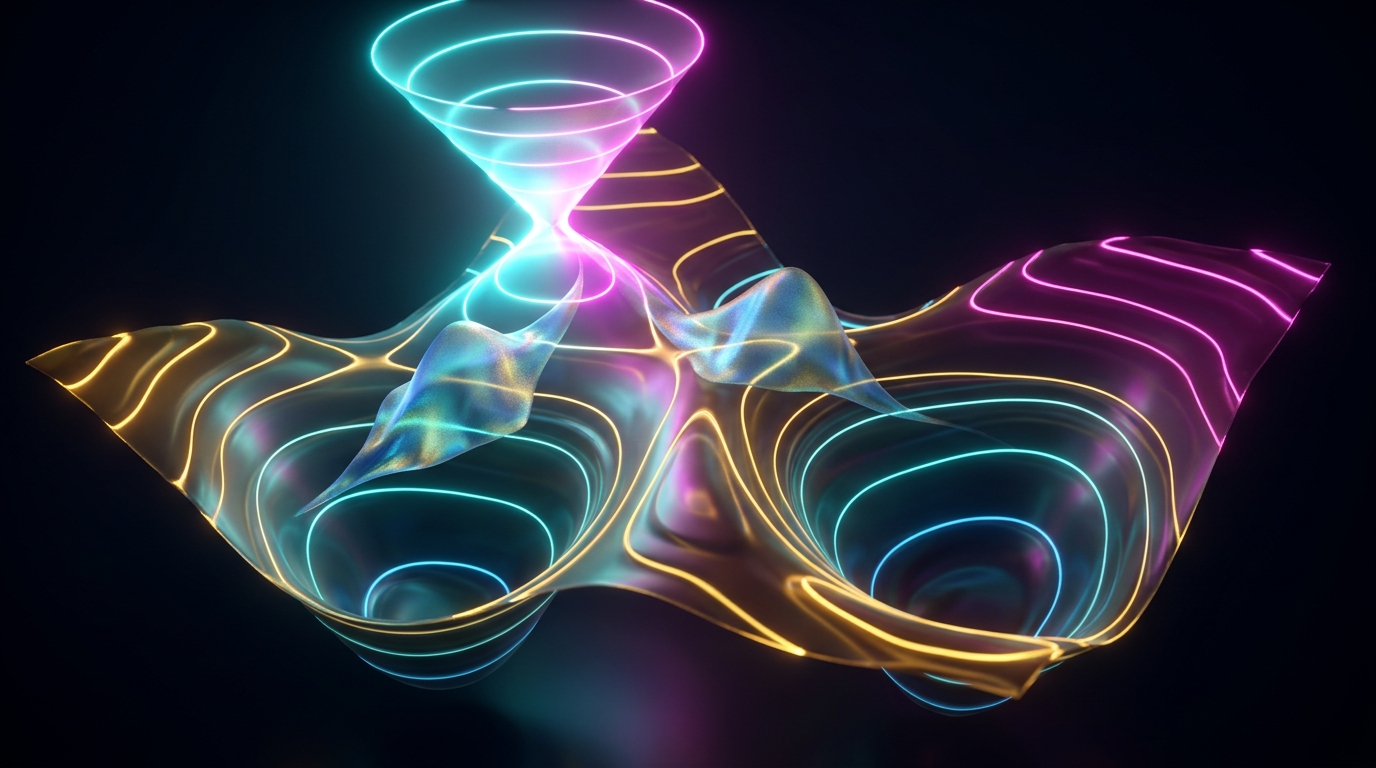
Ilustração 3D de uma Superfície de Energia Potencial mostrando dois poços profundos de mínimo, o ponto de sela central que os liga e um cone luminoso superior de interseção cónica entre estados excitado e fundamental

🌍 Ponto de Partida Químico e Ligação: Porque Precisamos Deste Capítulo?Chemical Starting Point & Connection: Why Do We Need This Chapter?

Ao longo do Bloco IV (Capítulos 13 a 17), aprendemos a resolver a estrutura eletrónica de uma molécula — seja com Hartree–Fock, $\text{CCSD(T)}$ ou Teoria do Funcional da Densidade (DFT). Mas todos esses cálculos tinham uma limitação silenciosa: assumiam que já sabíamos exatamente onde estão os núcleos no espaço 3D! Na vida real de um laboratório de Química Orgânica, Farmacêutica ou Bioquímica, quando desenhamos uma molécula nova num programa gráfico (como o Avogadro ou o ChemDraw 3D), as ligações que traçamos com o rato estão demasiado compridas, os anéis estão tensos e os átomos chocam uns com os outros. Se calcularmos a energia dessa estrutura «desenhada à mão», obteremos o valor de uma molécula deformada que não existe na Natureza. Throughout Block IV (Chapters 13 to 17), we learned how to solve the electronic structure of a molecule — whether via Hartree–Fock, $\text{CCSD(T)}$, or Density Functional Theory (DFT). Yet all of those calculations shared a silent limitation: they assumed we already knew the exact 3D positions of the nuclei! In the daily life of an Organic, Pharmaceutical, or Biochemistry lab, when you sketch a new molecule in a 3D builder (like Avogadro or ChemDraw 3D), the bonds you draw with your mouse are stretched, rings are strained, and atoms clash. Computing the energy of that hand-drawn sketch gives the energy of a distorted molecule that does not exist in Nature.

Mais importante ainda: um químico não quer apenas conhecer a forma estática de um reagente dentro de um frasco; quer descobrir como os átomos se reorganizam durante uma reação química, qual é a geometria exata do Estado de Transição ($\text{TS}^\ddagger$) — aquele instante fugaz de $10^{-13}$ segundos em que uma ligação velha se parte enquanto uma ligação nova nasce — e qual é a altura da barreira energética que decide se a reação ocorre à temperatura ambiente ou exige aquecimento a $150^\circ\text{C}$. Este Capítulo 18 ensina como transformamos o programa de Química Quântica num «GPS de montanha» capaz de caminhar sozinho pela Superfície de Energia Potencial até encontrar os vales (moléculas estáveis) e os passos de montanha (estados de transição). More importantly still, a chemist does not just want the static shape of a reactant sitting in a flask; we want to discover how atoms rearrange during a chemical reaction, what the exact geometry of the Transition State ($\text{TS}^\ddagger$) looks like — that fleeting $10^{-13}$-second instant where an old bond breaks while a new bond forms — and how high the energy barrier is that decides whether a reaction runs at room temperature or requires heating to $150^\circ\text{C}$. Chapter 18 shows how we turn a Quantum Chemistry program into a "mountain GPS" that walks across the Potential Energy Surface to locate valleys (stable molecules) and mountain passes (transition states).

18.1 Sentir a Inclinação da Montanha: O Teorema de Hellmann–Feynman e a Origem Física das Forças de Pulay (1969) 18.1 Feeling the Mountain Slope: The Hellmann–Feynman Theorem & the Physical Origin of Pulay Forces (1969)

A Ideia Física Imagine que soltamos uma molécula com uma geometria inicial distorcida — por exemplo, uma molécula de água onde esticámos uma ligação $\text{O–H}$ para $1.30\text{ Å}$ em vez dos seus $0.96\text{ Å}$ naturais. Tal como uma mola esticada, a nuvem eletrónica puxa imediatamente o núcleo de Hidrogénio de volta para perto do Oxigénio. Em Física e em Química, essa tendência de a energia baixar quando movemos um átomo mede-se pela inclinação (primeira derivada) da Superfície de Energia Potencial, a que chamamos o Vetor Gradiente Nuclear $\mathbf{g}_A$. The Physical Idea Imagine releasing a molecule from a distorted starting geometry — say, a water molecule where one $\text{O–H}$ bond has been stretched to $1.30\text{ Å}$ instead of its natural $0.96\text{ Å}$. Just like a stretched spring, the electron cloud immediately pulls the Hydrogen nucleus back toward Oxygen. In Physics and Chemistry, that tendency for the energy to drop when an atom moves is measured by the slope (first derivative) of the Potential Energy Surface, called the Nuclear Gradient Vector $\mathbf{g}_A$.

A relação entre o gradiente $\mathbf{g}_A$ e a força mecânica real $\mathbf{F}_A$ que empurra o núcleo $A$ difere apenas num sinal menos: o gradiente aponta sempre para o lado onde a energia sobe (encosta acima), enquanto a força física $\mathbf{F}_A = -\mathbf{g}_A$ empurra os átomos para onde a energia desce (encosta abaixo, em direção ao vale de equilíbrio): The relationship between the gradient $\mathbf{g}_A$ and the actual mechanical force $\mathbf{F}_A$ pushing nucleus $A$ differs only by a minus sign: the gradient always points in the direction where energy rises (uphill), whereas the physical force $\mathbf{F}_A = -\mathbf{g}_A$ pushes atoms toward lower energy (downhill, toward the equilibrium valley):

DEFINIÇÃO DE GRADIENTE NUCLEAR $\mathbf{g}_A$ E FORÇA ATÓMICA $\mathbf{F}_A$DEFINITION OF NUCLEAR GRADIENT $\mathbf{g}_A$ & ATOMIC FORCE $\mathbf{F}_A$ $$\mathbf{g}_A(\mathbf{R}) \equiv \nabla_{\mathbf{R}_A} E_{\text{BO}}(\mathbf{R}) = \left(\frac{\partial E_{\text{BO}}}{\partial X_A},\, \frac{\partial E_{\text{BO}}}{\partial Y_A},\, \frac{\partial E_{\text{BO}}}{\partial Z_A}\right)^{\!\mathsf{T}} = -\mathbf{F}_A(\mathbf{R})$$

🗣️ O que esta equação significa sem matemática:What this equation means without math:
Para cada átomo $A$ da molécula, o computador calcula três números $(g_{X_A}, g_{Y_A}, g_{Z_A})$ que respondem à pergunta: «Se eu empurrar este átomo um milésimo de Angström para a direita, para a frente ou para cima, a energia sobe ou desce?» Quando esses três números chegam a zero em todos os átomos ($\mathbf{g}_A = \mathbf{0}$), nenhum átomo sente qualquer força a puxá-lo — chegámos a um Ponto Estacionário! For every atom $A$ in the molecule, the computer evaluates three numbers $(g_{X_A}, g_{Y_A}, g_{Z_A})$ that answer the question: "If I nudge this atom by a thousandth of an Angstrom to the right, forward, or up, does the energy rise or fall?" When all three numbers reach zero on every atom ($\mathbf{g}_A = \mathbf{0}$), no atom feels any net pull — we have reached a Stationary Point!

Mas como é que o computador calcula estas forças sem ter de mover cada átomo um por um (o que exigiria centenas de cálculos SCF para uma única molécula)? Na década de 1930, Hans Hellmann e Richard Feynman demonstraram um resultado de enorme elegância física: uma vez conhecida a densidade eletrónica exata $\rho(\mathbf{r})$, a força que atua sobre um núcleo seria simplesmente a força eletrostática clássica (Lei de Coulomb) exercida pela nuvem negativa $\rho(\mathbf{r})$ e pelos outros núcleos! Porém, em 1969, o químico húngaro Péter Pulay descobriu que nos programas reais de Química Quântica existe uma força extra crucial — as célebres Forças de Pulay: Yet how does the computer evaluate these forces without nudging every atom one by one (which would require hundreds of SCF calculations for a single step)? In the 1930s, Hans Hellmann and Richard Feynman proved a result of remarkable physical elegance: once the exact electron density $\rho(\mathbf{r})$ is known, the force on a nucleus would simply be the classical electrostatic (Coulomb) force exerted by the negative cloud $\rho(\mathbf{r})$ and the other nuclei! However, in 1969, Hungarian chemist Péter Pulay discovered that in real Quantum Chemistry software there is a crucial extra contribution — the famous Pulay Forces:

⛺ Analogia Intuitiva: Porque Aparecem as Forças de Pulay? («As Estacas da Tenda que Viajam na Mochila»)Intuitive Analogy: Where Do Pulay Forces Come From? ("The Tent Poles Riding in the Backpack")
Imagine que está a medir o vento numa montanha usando uma tenda de pano (as nossas funções de base Gaussianas $\chi_\mu(\mathbf{r} - \mathbf{R}_A)$). Se a tenda estivesse pregada ao chão da montanha de forma independente de si (como acontece nas bases de Ondas Planas ou numa base infinita completa), ao dar um passo sentiria apenas a inclinação real do terreno (a Força de Hellmann–Feynman). Mas nos programas moleculares (ORCA, Gaussian), cada átomo $A$ carrega as suas próprias funções de base Gaussianas centradas às costas! Quando o núcleo $A$ se move $\Delta\mathbf{R}_A$, ele arrasta consigo as funções matemáticas que descrevem a nuvem eletrónica. A variação de energia causada por arrastar as próprias funções de base finitas com o núcleo é exatamente a Força de Pulay! Imagine measuring the slope of a mountain while carrying a canvas tent (our Gaussian basis functions $\chi_\mu(\mathbf{r} - \mathbf{R}_A)$). If the tent were staked permanently to the mountain grid independently of you (as in Plane-Wave basis sets or an infinite complete basis), taking a step would only register the true terrain slope (the Hellmann–Feynman Force). But in molecular codes (ORCA, Gaussian), each atom $A$ carries its own atom-centered Gaussian basis functions on its back! When nucleus $A$ moves by $\Delta\mathbf{R}_A$, it drags the mathematical functions describing the electron cloud along with it. The energy change caused by dragging finite basis functions along with the nucleus is precisely the Pulay Force!

📐 Dedução Matemática Guiada: Do Teorema de Hellmann–Feynman às Forças de PulayGuided Mathematical Derivation: From the Hellmann–Feynman Theorem to Pulay Forces

Passo 1 (Derivada do Valor Esperado da Energia): Aplicando a regra de derivação do produto a $E(\mathbf{R}) = \langle \Psi(\mathbf{R}) | \hat{H}(\mathbf{R}) | \Psi(\mathbf{R}) \rangle$: Step 1 (Derivative of the Energy Expectation Value): Applying the product rule of differentiation to $E(\mathbf{R}) = \langle \Psi(\mathbf{R}) | \hat{H}(\mathbf{R}) | \Psi(\mathbf{R}) \rangle$:

$$\frac{\partial E}{\partial \mathbf{R}_A} = \left\langle \Psi \left| \frac{\partial \hat{H}}{\partial \mathbf{R}_A} \right| \Psi \right\rangle + \left\langle \frac{\partial \Psi}{\partial \mathbf{R}_A} \left| \hat{H} \right| \Psi \right\rangle + \left\langle \Psi \left| \hat{H} \right| \frac{\partial \Psi}{\partial \mathbf{R}_A} \right\rangle$$

Passo 2 (Termo Eletrostático de Hellmann–Feynman): O primeiro termo deriva apenas o operador Hamiltoniano $\hat{H}$ (onde $\mathbf{R}_A$ entra na atração eletrão-núcleo $V_{ne}$ e na repulsão núcleo-núcleo $V_{nn}$), dando a força eletrostática clássica pura da nuvem $\rho(\mathbf{r})$: Step 2 (Hellmann–Feynman Electrostatic Term): The first term differentiates only the Hamiltonian operator $\hat{H}$ (where $\mathbf{R}_A$ enters the electron-nuclear attraction $V_{ne}$ and nuclear repulsion $V_{nn}$), yielding the pure electrostatic force of the electron cloud $\rho(\mathbf{r})$:

$$\left\langle \Psi \left| \frac{\partial \hat{H}}{\partial \mathbf{R}_A} \right| \Psi \right\rangle = -Z_A \int \rho(\mathbf{r})\,\frac{\mathbf{r} - \mathbf{R}_A}{|\mathbf{r} - \mathbf{R}_A|^3}\,d\mathbf{r} + \sum_{B \ne A} Z_A Z_B \frac{\mathbf{R}_A - \mathbf{R}_B}{|\mathbf{R}_A - \mathbf{R}_B|^3}$$

Passo 3 (Termo de Pulay para Bases Centradas nos Átomos): Como $\phi_i(\mathbf{r}) = \sum_\mu c_{\mu i}\chi_\mu(\mathbf{r} - \mathbf{R}_A)$, no fim do ciclo SCF a energia é estacionária face aos coeficientes ($\partial E / \partial c_{\mu i} = 0$), mas as funções de base $\chi_\mu$ e a sua matriz de sobreposição $S_{\mu\nu}$ mudam com $\mathbf{R}_A$, gerando as Forças de Pulay (onde $W_{\mu\nu} = \sum_i^{\text{occ}} n_i \varepsilon_i c_{\mu i} c_{\nu i}$ é a matriz de densidade ponderada pela energia): Step 3 (Pulay Term for Atom-Centered Basis Sets): Because $\phi_i(\mathbf{r}) = \sum_\mu c_{\mu i}\chi_\mu(\mathbf{r} - \mathbf{R}_A)$, at SCF convergence the energy is stationary with respect to the orbital coefficients ($\partial E / \partial c_{\mu i} = 0$), but the basis functions $\chi_\mu$ and their overlap matrix $S_{\mu\nu}$ shift with $\mathbf{R}_A$, producing the Pulay Forces (where $W_{\mu\nu} = \sum_i^{\text{occ}} n_i \varepsilon_i c_{\mu i} c_{\nu i}$ is the energy-weighted density matrix):

$$\begin{gathered} \frac{\partial E_{\text{SCF}}}{\partial \mathbf{R}_A} = \underbrace{\left\langle \Psi \left| \frac{\partial \hat{H}}{\partial \mathbf{R}_A} \right| \Psi \right\rangle}_{\text{Força de Hellmann–Feynman}} + \underbrace{\sum_{\mu\nu} P_{\mu\nu}\frac{\partial h_{\mu\nu}}{\partial \mathbf{R}_A} + \frac{1}{2}\sum_{\mu\nu\lambda\sigma} \Gamma_{\mu\nu\lambda\sigma}\frac{\partial (\mu\nu|\lambda\sigma)}{\partial \mathbf{R}_A} - \sum_{\mu\nu} W_{\mu\nu}\frac{\partial S_{\mu\nu}}{\partial \mathbf{R}_A}}_{\text{Forças de Pulay (Derivadas das Funções de Base que se Movem com o Núcleo } A\text{)}} \end{gathered}$$

$$\begin{gathered} \frac{\partial E_{\text{SCF}}}{\partial \mathbf{R}_A} = \underbrace{\left\langle \Psi \left| \frac{\partial \hat{H}}{\partial \mathbf{R}_A} \right| \Psi \right\rangle}_{\text{Hellmann–Feynman Force}} + \underbrace{\sum_{\mu\nu} P_{\mu\nu}\frac{\partial h_{\mu\nu}}{\partial \mathbf{R}_A} + \frac{1}{2}\sum_{\mu\nu\lambda\sigma} \Gamma_{\mu\nu\lambda\sigma}\frac{\partial (\mu\nu|\lambda\sigma)}{\partial \mathbf{R}_A} - \sum_{\mu\nu} W_{\mu\nu}\frac{\partial S_{\mu\nu}}{\partial \mathbf{R}_A}}_{\text{Pulay Forces (Derivatives of Basis Functions Moving with Nucleus } A\text{)}} \end{gathered}$$

18.2 O Alpinista de Olhos Vendados: Otimização de Geometria por Newton–Raphson, Quasi-Newton (BFGS) e Coordenadas Internas 18.2 The Blindfolded Mountaineer: Geometry Optimization via Newton–Raphson, Quasi-Newton (BFGS) & Internal Coordinates

Agora que sabemos calcular a inclinação exata do terreno ($\mathbf{g}_k$) na geometria atual $\mathbf{q}_k$, como é que o computador decide Em que direção e de que tamanho deve ser o próximo passo $\Delta\mathbf{q}$ para chegar o mais depressa possível ao fundo do vale? Now that we know how to compute the exact slope ($\mathbf{g}_k$) at the current geometry $\mathbf{q}_k$, how does the computer decide both the direction and the step size $\Delta\mathbf{q}$ to reach the bottom of the valley as quickly as possible?

🥾 A Analogia do Alpinista de Olhos Vendados na Serra da Estrela:The Analogy of the Blindfolded Hiker in the Mountains:
Imagine um alpinista de olhos vendados no meio do nevoeiro da Serra da Estrela que quer descer até à lagoa no fundo do vale (o mínimo de energia), mas não consegue ver a paisagem inteira ao longe porque cada ponto da paisagem custa um cálculo quântico SCF caro. Tudo o que ele consegue sentir sob as botas no sítio onde está é:
1. A Altitude Atual $E(\mathbf{q}_k)$: a energia eletrónica da geometria atual.
2. A Inclinação sob os Pés $\mathbf{g}_k$: para que lado o chão desce (o gradiente analítico).
3. A Curvatura do Terreno $\mathbf{H}_k$ (Matriz Hessiana): se o chão está a ficar mais plano (perto do fundo do vale, exigindo um passo moderado e certeiro) ou se está numa parede muito côncava. Se o alpinista usar apenas a inclinação (método de Steepest Descent), andará aos ziguezagues durante centenas de passos; se usar também a curvatura (método de Newton–Raphson / Quasi-Newton BFGS), aproxima o vale por uma tigela parabólica e salta quase diretamente para o fundo em $10\text{ a }20$ passos! Picture a blindfolded hiker in thick mountain fog trying to walk down to the lake at the bottom of a valley (the energy minimum), unable to see the whole landscape from afar because every point costs an expensive SCF calculation. All the hiker can feel right under their boots is:
1. Current Altitude $E(\mathbf{q}_k)$: the electronic energy at the current geometry.
2. Slope Underfoot $\mathbf{g}_k$: which way leads downhill (the analytical gradient).
3. Terrain Curvature $\mathbf{H}_k$ (Hessian Matrix): how rapidly the slope is flattening out. If the hiker uses only the slope (Steepest Descent), they will zig-zag down narrow canyons for hundreds of steps; if they also use the curvature (Newton–Raphson / Quasi-Newton BFGS), they approximate the valley as a parabolic bowl and step to the bottom in just $10\text{–}20$ steps!

Matematicamente, aproximar a vizinhança da geometria atual $\mathbf{q}_k$ por uma tigela quadrática (série de Taylor de 2.ª ordem) e procurar onde o gradiente se anula ($\mathbf{g}(\mathbf{q}_k + \Delta\mathbf{q}) = \mathbf{0}$) conduz à célebre Equação de Passo de Newton–Raphson, expressa na base dos vetores próprios $\mathbf{v}_i$ e valores próprios (curvaturas) $\lambda_i$ da matriz Hessiana $\mathbf{H}_k$: Mathematically, approximating the neighborhood of the current geometry $\mathbf{q}_k$ as a quadratic bowl (2nd-order Taylor expansion) and solving for where the gradient vanishes ($\mathbf{g}(\mathbf{q}_k + \Delta\mathbf{q}) = \mathbf{0}$) yields the celebrated Newton–Raphson Step Equation, written in the basis of the eigenvectors $\mathbf{v}_i$ and eigenvalues (curvatures) $\lambda_i$ of the Hessian matrix $\mathbf{H}_k$:

PASSO QUADRÁTICO DE NEWTON–RAPHSON E DECOMPOSIÇÃO NOS MODOS PRÓPRIOS DA HESSIANANEWTON–RAPHSON QUADRATIC STEP & HESSIAN EIGENMODE DECOMPOSITION $$\Delta\mathbf{q}_{\text{NR}} = -\mathbf{H}_k^{-1}\mathbf{g}_k = -\sum_{i=1}^{3M-6} \frac{\mathbf{v}_i^\mathsf{T}\mathbf{g}_k}{\lambda_i}\,\mathbf{v}_i$$

🗣️ Como ler esta equação para perceber porque é tão fácil achar mínimos e tão delicado achar Estados de Transição:How to read this equation to understand why finding minima is easy while finding Transition States is delicate:
• Para achar um Mínimo (! Opt com algoritmo BFGS): Queremos descer em todas as direções, por isso todas as curvaturas $\lambda_i$ têm de ser positivas ($\lambda_i > 0$). Como calcular a Hessiana exata em cada passo é caro, o algoritmo Quasi-Newton BFGS começa com uma Hessiana aproximada barata (regras empíricas de forças de ligação) e vai melhorando a curvatura a cada passo olhando para como o gradiente mudou ($\Delta\mathbf{g}_k = \mathbf{g}_{k+1} - \mathbf{g}_k$).
• Para achar um Estado de Transição $\text{TS}^\ddagger$ (! OptTS com algoritmo P-RFO / Bofill): Queremos subir a encosta ao longo de 1 única direção (a coordenada de reação onde $\lambda_1 \lt 0$) e descer em todas as outras $3M-7$ direções perpendiculares ($\lambda_{i\ge 2} > 0$). Por isso, na otimização de um $\text{TS}^\ddagger$, precisamos obrigatoriamente que a Hessiana inicial já conheça qual é o modo que tem curvatura negativa (usando %geom Calc_Hess true end no ORCA)! • To find a Minimum (! Opt with the BFGS algorithm): We want to step downhill in every direction, so all curvatures $\lambda_i$ must be positive ($\lambda_i > 0$). Because computing an exact Hessian at every step is costly, the Quasi-Newton BFGS algorithm starts from an inexpensive model Hessian and updates the curvature at each step from the change in gradients ($\Delta\mathbf{g}_k = \mathbf{g}_{k+1} - \mathbf{g}_k$).
• To find a Transition State $\text{TS}^\ddagger$ (! OptTS with the P-RFO / Bofill algorithm): We must walk uphill along 1 single direction (the reaction coordinate where $\lambda_1 \lt 0$) while stepping downhill along all other $3M-7$ perpendicular directions ($\lambda_{i\ge 2} > 0$). That is why, when optimizing a $\text{TS}^\ddagger$, the initial Hessian must accurately know which mode has negative curvature (by specifying %geom Calc_Hess true end in ORCA)!

18.3 A Matriz Hessiana Ponderada pela Massa $\mathbf{H}^{(m)}$ e as Frequências Vibracionais Harmónicas $\tilde{\nu}_k$ 18.3 The Mass-Weighted Hessian Matrix $\mathbf{H}^{(m)}$ & Harmonic Vibrational Frequencies $\tilde{\nu}_k$

Suponha que o seu cálculo de otimização no ORCA terminou com a mensagem feliz * THE OPTIMIZATION HAS CONVERGED *. Todas as forças sobre os átomos são agora nulas ($\mathbf{g} = \mathbf{0}$). Mas atenção: uma bola pousada no fundo de uma taça e uma bola equilibrada em cima do topo de um capacete têm ambas força zero! Como sabemos se o computador encontrou uma molécula estável (um vale) ou um estado de transição instável (um passo de montanha)? Suppose your optimization job in ORCA finishes with the happy banner * THE OPTIMIZATION HAS CONVERGED *. All forces on the atoms are now zero ($\mathbf{g} = \mathbf{0}$). Yet beware: a ball resting at the bottom of a bowl and a ball balanced precariously on top of a helmet both experience zero net force! How do we know whether the computer found a stable molecule (a valley) or an unstable transition state (a mountain pass)?

💬 Dúvida Frequente · Encontrei uma frequência imaginária pequena (por exemplo, −20 cm⁻¹) numa estrutura que devia ser um mínimo. É grave?💬 Student Q&A · I found a small imaginary frequency (e.g., −20 cm⁻¹) in a structure that should be a minimum. Is that serious?

Muitas vezes é ruído numérico, e não um verdadeiro estado de transição. Causas comuns: a otimização parou com critérios demasiado largos, a grelha de integração é grosseira, ou há uma rotação muito "mole", como a de um grupo metilo. O que fazer: veja que movimento corresponde à frequência (no Avogadro ou no Chemcraft), desloque a geometria um pouco nessa direção e volte a otimizar com critérios mais apertados (! TightOpt) e uma grelha mais fina. Se a frequência imaginária persistir e for grande, provavelmente está mesmo num ponto de sela.Often it is numerical noise, not a real transition state. Common causes: the optimization stopped with loose criteria, the integration grid is coarse, or there is a very "soft" rotation, such as a methyl group. What to do: look at which motion the frequency corresponds to (in Avogadro or Chemcraft), displace the geometry slightly along it, and re-optimize with tighter criteria (! TightOpt) and a finer grid. If the imaginary frequency persists and is large, you probably really are at a saddle point.

A única forma rigorosa é calcular a Matriz Hessiana (segundas derivadas da energia) através da palavra-chave ! Freq. Fisicamente, a segunda derivada $\frac{\partial^2 E}{\partial X_i \partial X_j}$ é a constante de força $k$ da mola química (Lei de Hooke). Dividindo pelas raízes quadradas das massas atómicas $\sqrt{m_i m_j}$ (porque um átomo leve de Hidrogénio vibra muito mais rápido do que um átomo pesado de Bromo sob a mesma força!) e diagonalizando a matriz, obtemos os $3M - 6$ modos normais de vibração $\mathbf{Q}_k$ e as suas frequências em números de onda $\tilde{\nu}_k$ ($\text{cm}^{-1}$): The only rigorous way is to compute the Hessian Matrix (second derivatives of the energy) via the ! Freq keyword. Physically, the second derivative $\frac{\partial^2 E}{\partial X_i \partial X_j}$ is the spring force constant $k$ of the chemical bond (Hooke's law). Dividing by the square roots of the atomic masses $\sqrt{m_i m_j}$ (since a light Hydrogen atom vibrates much faster than a heavy Bromine atom under the same force!) and diagonalizing the matrix yields the $3M - 6$ normal vibrational modes $\mathbf{Q}_k$ and their wavenumbers $\tilde{\nu}_k$ ($\text{cm}^{-1}$):

MATRIZ HESSIANA PONDERADA PELA MASSA E FREQUÊNCIAS VIBRACIONAIS EM NÚMEROS DE ONDA ($\text{cm}^{-1}$)MASS-WEIGHTED HESSIAN MATRIX & VIBRATIONAL FREQUENCIES IN WAVENUMBERS ($\text{cm}^{-1}$) $$H_{ij}^{(m)} = \frac{1}{\sqrt{m_i m_j}}\left(\frac{\partial^2 E_{\text{BO}}}{\partial X_i\,\partial X_j}\right)_{\!\mathbf{R}_0}, \qquad \mathbf{H}^{(m)}\mathbf{Q}_k = \lambda_k \mathbf{Q}_k, \qquad \tilde{\nu}_k = \frac{1}{2\pi c}\sqrt{\lambda_k} = \frac{1}{2\pi c}\sqrt{\frac{k_k}{\mu_k}}$$

🗣️ Porque é que uma curvatura negativa ($\lambda_1 \lt 0$) dá uma «Frequência Imaginária»?Why does a negative curvature ($\lambda_1 \lt 0$) produce an "Imaginary Frequency"?
Olhe para a raiz quadrada $\tilde{\nu}_k = \frac{1}{2\pi c}\sqrt{\lambda_k}$:
• No fundo de um vale (Mínimo): a superfície curva para cima em todas as direções ($\lambda_k > 0$), pelo que $\sqrt{\lambda_k}$ é um número real positivo. Todos os $3M-6$ modos têm frequências positivas ($\mathbf{n_{\text{imag}} = 0}$).
• No topo de uma barreira de reação (Estado de Transição $\text{TS}^\ddagger$): ao longo da coordenada de reação a superfície curva para baixo como uma colina ($\lambda_1 \lt 0$). A raiz quadrada de um número negativo é um número imaginário puro $\sqrt{-|\lambda_1|} = i\sqrt{|\lambda_1|}$! Nos ficheiros de output do ORCA e do Gaussian, esta frequência imaginária aparece impressa com um sinal menos à frente (por exemplo, -452.3 cm**-1). Um verdadeiro Estado de Transição tem exatamente $1$ frequência imaginária ($\mathbf{n_{\text{imag}} = 1}$)! Look closely at the square root $\tilde{\nu}_k = \frac{1}{2\pi c}\sqrt{\lambda_k}$:
• At the bottom of a valley (Minimum): the surface curves upward in every direction ($\lambda_k > 0$), so $\sqrt{\lambda_k}$ is a positive real number. All $3M-6$ modes have positive frequencies ($\mathbf{n_{\text{imag}} = 0}$).
• At the top of a reaction barrier (Transition State $\text{TS}^\ddagger$): along the reaction coordinate the surface curves downward like the crest of a hill ($\lambda_1 \lt 0$). The square root of a negative number is a purely imaginary number $\sqrt{-|\lambda_1|} = i\sqrt{|\lambda_1|}$! In ORCA and Gaussian output files, this imaginary frequency is printed with a minus sign in front (e.g., -452.3 cm**-1). A true Transition State has exactly $1$ imaginary frequency ($\mathbf{n_{\text{imag}} = 1}$)!

Tipo de Ponto Estacionário ($\mathbf{g} = \mathbf{0}$)Stationary Point Type ($\mathbf{g} = \mathbf{0}$)	Índice da Hessiana ($n_{\text{imag}}$)Hessian Index ($n_{\text{imag}}$)	Sinal dos Valores Próprios $\lambda_k$Sign of Eigenvalues $\lambda_k$	Significado Químico e Ação Prática no ORCA/GaussianChemical Meaning & Practical Action in ORCA/Gaussian
Mínimo Local ou GlobalLocal or Global Minimum	$\mathbf{n_{\text{imag}} = 0}$	Todos os $3M-6$ valores próprios $\lambda_k > 0$ (todas as $\tilde{\nu}_k$ reais positivas).All $3M-6$ eigenvalues $\lambda_k > 0$ (all $\tilde{\nu}_k$ real and positive).	Espécie quimicamente estável (reagente, intermediário de reação ou produto). Pode prosseguir para o cálculo da energia livre de Gibbs $G^\circ(T)$.Chemically stable species (reactant, reaction intermediate, or product). Safe to proceed to Gibbs free energy $G^\circ(T)$ evaluation.
Ponto de Sela de 1.ª Ordem (Estado de Transição $\text{TS}^\ddagger$)1st-Order Saddle Point (Transition State $\text{TS}^\ddagger$)	$\mathbf{n_{\text{imag}} = 1}$	Exatamente $1$ valor próprio negativo ($\lambda_1 \lt 0 \implies \tilde{\nu}_1 = i\|\tilde{\nu}^\ddagger\|$, impresso como `-452.3 cm-1`) e $3M-7$ positivos.Strictly $1$ negative eigenvalue ($\lambda_1 \lt 0 \implies \tilde{\nu}_1 = i\|\tilde{\nu}^\ddagger\|$, printed as `-452.3 cm``-1`) and $3M-7$ positive ones.	Topo de uma barreira elementar de reação. Obrigatório animar o vetor próprio $\mathbf{Q}_1$ no Chemcraft/Avogadro e correr um cálculo `! IRC` para provar que liga o reagente ao produto pretendido!Apex of an elementary reaction barrier. Mandatory to animate eigenvector $\mathbf{Q}_1$ in Chemcraft/Avogadro and run an `! IRC` calculation to prove it connects the intended reactant and product!
Ponto de Sela de Ordem Superior ($n_{\text{imag}} \ge 2$)Higher-Order Saddle Point ($n_{\text{imag}} \ge 2$)	$\mathbf{n_{\text{imag}} \ge 2}$	Dois ou mais valores próprios negativos ($\lambda_1 \lt 0, \lambda_2 \lt 0, \dots$).Two or more negative eigenvalues ($\lambda_1 \lt 0, \lambda_2 \lt 0, \dots$).	Geometria inválida para termoquímica ou cinética! Pelo Teorema de Murrell–Laidler (1968), o caminho de menor energia entre dois vales passa por um ponto de sela de 1.ª ordem ($n_{\text{imag}}=1$). Perturbe a geometria ao longo do modo imaginário espúrio (ex.: rotação de grupo $-\text{CH}_3$), suba a grelha para `DefGrid3` e reotimize!Invalid geometry for thermochemistry or kinetics! By the Murrell–Laidler theorem (1968), the minimum-energy path between two valleys passes through a 1st-order saddle point ($n_{\text{imag}}=1$). Displace the geometry along the spurious imaginary mode (e.g., $-\text{CH}_3$ rotation), tighten the grid to `DefGrid3`, and re-optimize!

18.4 Como Encontrar e Provar um Estado de Transição ($\text{TS}^\ddagger$): Banda Elástica (`NEB-TS`) e Coordenada Intrínseca de Reação (`IRC` de Fukui) 18.4 How to Find and Prove a Transition State ($\text{TS}^\ddagger$): Nudged Elastic Band (`NEB-TS`) & Fukui's Intrinsic Reaction Coordinate (`IRC`)

No trabalho prático de investigação, encontrar o Estado de Transição ($\text{TS}^\ddagger$) é a etapa mais emocionante — e por vezes a mais desafiante — de um estudo de mecanismo reacional. Porque é que não basta desenhar uma estrutura «a olho» e correr ! OptTS? Porque o algoritmo de subida de sela (P-RFO) só sabe qual direção deve subir se a estrutura inicial já estiver suficientemente perto do passo de montanha onde a ligação que se quebra/forma tem curvatura negativa! In day-to-day research, locating the Transition State ($\text{TS}^\ddagger$) is the most exciting — and sometimes most challenging — part of a mechanistic study. Why can't we just eyeball a structure and run ! OptTS? Because the saddle-point climb algorithm (P-RFO) only knows which direction to walk uphill if the starting geometry is already close enough to the mountain pass where the breaking/forming bond has negative curvature!

🧪 Paralelo Real de Laboratório: Porque É Obrigatório Correr o Cálculo IRC Antes de Publicar um Mecanismo?Real Laboratory Parallel: Why Is Running an IRC Calculation Mandatory Before Publishing a Mechanism? Imagine que está a estudar uma reação enzimática ou organocatalítica onde um substrato pode sofrer substituição nucleofílica ($\text{S}_{\text{N}}2$) ou eliminação ($\text{E2}$). Você otimiza um estado de transição, corre ! Freq e vê exatamente $1$ frequência imaginária (-410 cm**-1). Parece perfeito! Mas quando corre o cálculo ! IRC (que empurra ligeiramente a molécula para a frente e para trás ao longo desse modo imaginário e a deixa escorregar encosta abaixo sem velocidade inicial), descobre que um dos lados desce para um intermediário completamente diferente daquele que imaginava! Na literatura moderna (JACS, Angewandte Chemie, Nature Chemistry), um $\text{TS}^\ddagger$ só é considerado provado quando a curva IRC demonstra inequivocamente que o vale $s \lt 0$ é o reagente e o vale $s > 0$ é o produto. Imagine studying an enzymatic or organocatalytic reaction where a substrate can undergo either nucleophilic substitution ($\text{S}_{\text{N}}2$) or elimination ($\text{E2}$). You optimize a transition state, run ! Freq, and see exactly $1$ imaginary frequency (-410 cm**-1). It looks perfect! Yet when you run an ! IRC job (which nudges the molecule forward and backward along that imaginary mode and lets it slide downhill with zero initial velocity), you discover that one side slides into an unexpected intermediate rather than your intended reactant! In modern journals (JACS, Angewandte Chemie, Nature Chemistry), a $\text{TS}^\ddagger$ is only proven once the IRC curve confirms that the $s \lt 0$ valley is the reactant and the $s > 0$ valley is the product.

💬 Dúvida de Estudante: «E se o meu cálculo de mínimo (! Opt Freq) terminar com uma pequena frequência imaginária de -18 cm-1 correspondente à rotação de um grupo metilo ($-\text{CH}_3$)? Posso ignorá-la?»Student Question: "What if my minimum optimization (! Opt Freq) finishes with a tiny imaginary frequency of -18 cm-1 corresponding to a methyl ($-\text{CH}_3$) rotation? Can I ignore it?" Não deve ignorá-la! Mesmo uma pequena frequência imaginária de $-15\text{ a }-30\text{ cm}^{-1}$ significa que o grupo metilo ficou estacionado no topo eclipsado da sua barreira de rotação (ou que a grelha numérica era demasiado grossa), perdendo um modo vibracional real que contribui com $\approx 0.6\text{ kcal/mol}$ para a entropia $-TS$! A solução no ORCA é simples: aumente a grelha numérica para ! DefGrid3 TightOpt (ou desloque ligeiramente as coordenadas ao longo desse modo no Chemcraft/Avogadro) e reotimize até obter $n_{\text{imag}} = 0$. Do not ignore it! Even a small imaginary mode of $-15\text{ to }-30\text{ cm}^{-1}$ means the methyl group got stuck in an eclipsed rotational conformation (or that the integration grid was too coarse), costing you a real low-frequency mode that contributes $\approx 0.6\text{ kcal/mol}$ to the $-TS$ entropy term! The fix in ORCA is simple: tighten the grid with ! DefGrid3 TightOpt (or slightly displace coordinates along that mode in Chemcraft/Avogadro) and re-optimize until $n_{\text{imag}} = 0$.

🔬 Interativo 18.1Interactive 18.1 Explorador da Superfície de Energia Potencial, Valores Próprios da Hessiana e Caminho IRC ($\text{Cl}^- + \text{CH}_3\text{Br} \to \text{CH}_3\text{Cl} + \text{Br}^-$) Potential Energy Surface, Hessian Eigenvalue & IRC Path Explorer ($\text{Cl}^- + \text{CH}_3\text{Br} \to \text{CH}_3\text{Cl} + \text{Br}^-$)

Arraste o cursor da coordenada de reação $s$ desde o vale dos reagentes ($s = -4.0$) até ao vale dos produtos ($s = +4.0$), passando pelo Estado de Transição bipiramidal trigonal ($s = 0.0$), e observe como a inclinação $g_s$, as distâncias $\text{C–Cl} / \text{C–Br}$ e a frequência vibracional mudam em tempo real: Drag the reaction coordinate slider $s$ from the reactant valley ($s = -4.0$) across the trigonal-bipyramidal Transition State ($s = 0.0$) to the product valley ($s = +4.0$), and watch how the slope $g_s$, the $\text{C–Cl} / \text{C–Br}$ bond distances, and the vibrational frequency evolve in real time:

🎯 O Que Se Pretende Fazer Neste Simulador e Porquê What This Simulator Does & Why It Matters

Objetivo: Explorar a Superfície de Energia Potencial (PES) e a Coordenada Intrínseca de Reação (IRC) de uma substituição nucleofílica $\text{S}_{\text{N}}2$ (Capítulo 18), relacionando o declive (gradiente) e a curvatura (frequências reais vs. $1$ frequência imaginária da Hessiana) com os pontos estacionários. Goal: Explore the Potential Energy Surface (PES) and Intrinsic Reaction Coordinate (IRC) of an $\text{S}_{\text{N}}2$ nucleophilic substitution (Chapter 18), connecting the slope (gradient) and curvature (real frequencies vs. $1$ imaginary Hessian frequency) to stationary points.

Coordenada Intrínseca de Reação $s$ ($\text{amu}^{1/2}\text{Bohr}$):Intrinsic Reaction Coordinate $s$ ($\text{amu}^{1/2}\text{Bohr}$): s = 0.00 (Estado de Transição TS‡)s = 0.00 (Transition State TS‡)

ℹ️ Explicação deste seletor / controlo (clique para abrir)ℹ️ Explanation of this selector / control (click to open)

O que controla: Move o sistema ao longo da Coordenada Intrínseca de Reação (IRC) $s$ de Fukui desde os reagentes ($s = -4.0$) até aos produtos ($s = +4.0$), passando pelo Estado de Transição $\text{TS}^\ddagger$ ($s = 0.0$).
O que observar: Siga a evolução do gradiente $g_s = dE/ds$ (que se anula nos mínimos e no $\text{TS}^\ddagger$) e o número de frequências imaginárias $n_{\text{imag}}$ da matriz Hessiana ($0$ nos mínimos vs. $1$ no ponto de sela $\text{TS}^\ddagger$).What it controls: Moves the system along Fukui's Intrinsic Reaction Coordinate (IRC) $s$ from reactants ($s = -4.0$) through the Transition State $\text{TS}^\ddagger$ ($s = 0.0$) to products ($s = +4.0$).
What to observe: Track the energy gradient $g_s = dE/ds$ (zero at minima and $\text{TS}^\ddagger$) and the Hessian imaginary frequency count $n_{\text{imag}}$ ($0$ at minima vs. $1$ at the $\text{TS}^\ddagger$ saddle point).

Saltar para um ponto crítico da reação $\text{S}_{\text{N}}2$:Jump to a critical point along the $\text{S}_{\text{N}}2$ reaction:

ℹ️ Explicação deste seletor / controlo (clique para abrir)ℹ️ Explanation of this selector / control (click to open)

O que faz este seletor: Salta diretamente para os 3 pontos estacionários críticos da reação $\text{S}_{\text{N}}2$ (Complexo de Reagentes, Estado de Transição Bipiramidal $\text{TS}^\ddagger$ ou Complexo de Produtos).What this selector does: Jumps directly to the 3 critical stationary points along the $\text{S}_{\text{N}}2$ reaction path (Reactant Complex, Bipyramidal Transition State $\text{TS}^\ddagger$, or Product Complex).

Energia Relativa $\Delta E(s)$Relative Energy $\Delta E(s)$

+13.40 kcal/mol

Gradiente $g_s = dE/ds$Gradient $g_s = dE/ds$

0.000 kcal/(mol·s)

Distâncias $R_{\text{C–Cl}} \;/\; R_{\text{C–Br}}$Distances $R_{\text{C–Cl}} \;/\; R_{\text{C–Br}}$

2.31 Å / 2.46 Å

Curvatura $\lambda_1$ e Frequência $\tilde{\nu}_1$Curvature $\lambda_1$ & Frequency $\tilde{\nu}_1$

452i cm⁻¹ (TS‡, n_imag=1)

📌 Mensagens-Chave para o Químico (Resumo sem Matemática) — Capítulo 18Key Takeaways for Chemists (Math-Free Summary) — Chapter 18

1. Forças Analíticas ($\mathbf{F}_A = -\mathbf{g}_A$): Um programa de Química Quântica otimiza uma estrutura 3D calculando a força exata sobre cada átomo (soma da força eletrostática de Hellmann–Feynman com as forças de Pulay das funções de base que viajam agarradas aos núcleos) até todas as forças se anularem ($\mathbf{g} = \mathbf{0}$).1. Analytical Forces ($\mathbf{F}_A = -\mathbf{g}_A$): A Quantum Chemistry program optimizes a 3D structure by evaluating the exact force on each atom (sum of the Hellmann–Feynman electrostatic force and the Pulay forces of atom-centered basis functions) until all forces vanish ($\mathbf{g} = \mathbf{0}$).
2. A Regra das Frequências Imaginárias ($n_{\text{imag}}$): Força zero não garante estabilidade! É obrigatório calcular a Matriz Hessiana (! Freq): uma molécula estável (mínimo) tem $0$ frequências imaginárias; um Estado de Transição ($\text{TS}^\ddagger$) tem exatamente $1$ frequência imaginária ao longo da ligação que se forma/quebra.2. The Imaginary Frequency Rule ($n_{\text{imag}}$): Zero force does not guarantee stability! Evaluating the Hessian matrix (! Freq) is mandatory: a stable molecule (minimum) has $0$ imaginary frequencies; a Transition State ($\text{TS}^\ddagger$) has exactly $1$ imaginary frequency along the forming/breaking bond.
3. Validação por NEB-TS e IRC: Para encontrar estados de transição complexos, use ! NEB-TS entre reagente e produto; depois de encontrar o $\text{TS}^\ddagger$, confirme sempre com ! IRC que os dois lados da barreira escorregam para o reagente e produto esperados.3. Validation via NEB-TS and IRC: To locate complex transition states, run ! NEB-TS between reactant and product; once the $\text{TS}^\ddagger$ is found, always confirm with ! IRC that the two sides of the barrier slide down to the intended reactant and product valleys.

🎯 Questionário de Conceitos Fundamentais — Exploração da Superfície de Energia Potencial (PES): Gradientes Analíticos, Otimização de Geometria, Estados de Transição ($\text{TS}^\ddagger$), Matriz Hessiana e Coordenada Intrínseca de Reação (IRC)Core Concepts Questionnaire — Exploring the Potential Energy Surface (PES): Analytical Gradients, Geometry Optimization, Transition States ($\text{TS}^\ddagger$), Hessian Matrix & Intrinsic Reaction Coordinate (IRC)

Questões acessíveis sobre os conceitos essenciais deste capítulo • Clique em «Outra Variante» ou «Feedback de Estudo» para saber o que estudar mais.Accessible questions on this chapter's essential concepts • Click "Swap Variant" or "Study Feedback" for personalized study guidance.

0 / 4 (0%)

🔗 Texto de Ligação para o Capítulo 19Bridge to Chapter 19

Agora que já sabemos obter a geometria 3D exata de qualquer molécula estável ou estado de transição na Superfície de Energia Potencial, surge a pergunta seguinte de qualquer químico: como é que os eletrões estão distribuídos dentro dessa estrutura 3D? Que átomos ficaram ricos em carga negativa (nucleofílicos) e que átomos ficaram deficientes em eletrões (eletrofílicos)? No Capítulo 19 vamos descobrir porque é que o momento dipolar e o Potencial Eletrostático Molecular são grandezas físicas reais, enquanto as famosas «cargas atómicas parciais» são modelos humanos que temos de saber escolher com cuidado! Now that we know how to obtain the exact 3D geometry of any stable molecule or transition state on the Potential Energy Surface, the next question every chemist asks is: how are the electrons distributed inside that 3D structure? Which atoms are electron-rich (nucleophilic) and which are electron-poor (electrophilic)? In Chapter 19 we will discover why the dipole moment and Molecular Electrostatic Potential are true physical observables, whereas partial atomic charges are human partitioning models that must be chosen with care!

📖 Síntese Pedagógica Acessível • Escada de Jacob da DFTAccessible Pedagogical Synthesis • Escada de Jacob da DFT 📜 Ver Módulo 0 (História & Evolução Completa) →View Module 0 (Full History & Evolution) →

📘 Conceito Principal Explicado: Equações de Kohn–Sham, a Escada de Jacob da DFT, Erro de Auto-Interação (SIE) e Dispersão D3(BJ)Core Concept Explained: Kohn–Sham Equations, Perdew's Jacob's Ladder, Self-Interaction Error (SIE), and D3(BJ) Dispersion

Na formulação de Kohn–Sham (1965), calculamos a energia cinética exata $T_s[\rho]$ de um sistema fictício de eletrões não-interagentes que possui exatamente a mesma densidade $\rho(\vec{r})$ do sistema real, concentrando todos os efeitos quânticos de muitos corpos num único termo: o funcional de troca-correlação $E_{\text{XC}}[\rho]$: In Kohn–Sham DFT (1965), a reference system of non-interacting orbitals reproduces the exact density $\rho(\vec{r})$, concentrating all many-body quantum effects into the exchange–correlation functional $E_{\text{XC}}[\rho]$:

💡 Intuição Física:Physical Intuition: Como os funcionais semilocais (LDA/GGA) não anulam perfeitamente a repulsão de Coulomb $J[\rho]$ de um eletrão consigo próprio (Erro de Auto-Interação, SIE), tendem a sobre-deslocalizar eletrões e a subestimar barreiras de reação ($\text{H}_3^\ddagger$), e não capturam forças de London a longa distância ($-C_6/R^6$) sem a correção de dispersão `D3(BJ)` ou funcionais híbridos range-separated! Because semilocal functionals (LDA/GGA) suffer from Self-Interaction Error (SIE), they underestimate reaction barriers and miss long-range London dispersion ($-C_6/R^6$) unless augmented with exact exchange (hybrids) and `D3(BJ)` dispersion corrections!

🌍 Curiosidade & Ligação ao Mundo Real: Porque é que a grafite do seu lápis escreve no papel e como o ORCA calcula proteínas inteirasCuriosity & Real-World Connection: Why pencil graphite writes on paper and how DLPNO-CCSD(T) reaches whole enzyme active sites

Dentro de cada folha de grafeno na ponta de um lápis, os átomos de carbono estão unidos por ligações covalentes $\sigma/\pi$ fortíssimas ($\sim 500\text{ kJ mol}^{-1}$). Mas entre folhas adjacentes (separadas por $3.35\text{ Å}$), a coesão provém exclusivamente de forças de dispersão de London! Um cálculo `B3LYP` puro sem correção de dispersão prevê erradamente que a grafite se desfaz sozinha (repulsiva!), enquanto `B3LYP-D3(BJ)` reproduz exatamente a energia de esfoliação experimental ($\sim 52\text{ meV/átomo}$) que permite à ponta do lápis deixar camadas de grafeno no papel! Within each graphene sheet of a pencil, carbon atoms are held by strong covalent bonds, while adjacent sheets ($3.35\text{ Å}$ apart) are held purely by London dispersion! Uncorrected `B3LYP` falsely predicts graphite sheets to repel each other, whereas `B3LYP-D3(BJ)` accurately recovers the interlayer binding energy that lets pencils write on paper!

🏛️ Mostrar Cientistas Pioneiros e Fotografias Históricas da Wikipedia relacionados com este Bloco (4 Cartões Ilustrados)Show Related Pioneer Scientists & Historical Wikipedia Photos (4 Illustrated Cards)

Nobel 1998 • Teoremas HK & Kohn–Sham DFTNobel 1998 • HK Theorems & Kohn–Sham DFT

Walter Kohn (1923–2016) ↗

Provou com Hohenberg (1964) e Sham (1965) que a densidade eletrónica tridimensional determina univocamente todas as propriedades do estado fundamental. Proved with Hohenberg (1964) and Sham (1965) that the 3D electron density uniquely determines all ground-state properties.

🌐 Artigo na Wikipedia ↗Wikipedia Article ↗

Escada de Jacob da DFT (PBE, B88, B3LYP)Jacob's Ladder of DFT (PBE, B88, B3LYP)

John P. Perdew & Axel D. Becke ↗

Arquitetaram a hierarquia sistemática de funcionais de densidade (LDA -> GGA -> meta-GGA -> Híbridos) que revolucionou a química e física do estado sólido. Architected the systematic hierarchy of density functionals (LDA -> GGA -> meta-GGA -> Hybrids) across chemistry and materials science.

🌐 Artigo na Wikipedia ↗Wikipedia Article ↗

Dispersão DFT-D3/D4 & GFN2-xTBDFT-D3/D4 Dispersion & GFN2-xTB

Stefan Grimme (n. 1963) ↗

Desenvolveu as correções de dispersão dependentes do ambiente químico (D3/D4) e os métodos quânticos tight-binding ultrarrápidos. Developed chemical-environment-dependent London dispersion corrections (D3/D4) and ultrafast GFN-xTB quantum methods.

🌐 Artigo na Wikipedia ↗Wikipedia Article ↗

Bases def2, TURBOMOLE, ORCA & DLPNO-CCSD(T)def2 Basis Sets, ORCA & DLPNO-CCSD(T)

Reinhart Ahlrichs & Frank Neese ↗

Criaram as famílias de bases balanceadas def2-SVP/TZVP e o método DLPNO-CCSD(T) de escalamento linear para precisão Coupled Cluster em grandes moléculas. Created the balanced def2-SVP/TZVP basis sets and linear-scaling DLPNO-CCSD(T) for gold-standard accuracy in large systems.

🌐 Artigo na Wikipedia ↗Wikipedia Article ↗

Propriedades Eletrónicas, Momentos Multipolares, Potencial Eletrostático Molecular (MEP) e Análise Populacional (Observáveis vs. Cargas Atómicas Parciais) Electronic Properties, Multipole Moments, Molecular Electrostatic Potential (MEP) & Population Analysis (Observables vs. Partial Atomic Charges)

Porque é que o momento dipolar e o potencial eletrostático são factos experimentais da Natureza, enquanto as cargas parciais atómicas (Mulliken, NBO, QTAIM, RESP) são fronteiras desenhadas por humanos sobre uma nuvem eletrónica contínua. Why the dipole moment and electrostatic potential are experimental facts of Nature, whereas partial atomic charges (Mulliken, NBO, QTAIM, RESP) are human-drawn borders across a continuous electron cloud.

🌍 Ponto de Partida Químico e Ligação: Porque Precisamos Deste Capítulo?Chemical Starting Point & Connection: Why Do We Need This Chapter?

Desde a primeira aula de Química Orgânica ou Química Geral, os químicos pensam e desenham reações usando cargas parciais ($\delta^+$ e $\delta^-$): dizemos que numa carbonila ($\text{C=O}$) o carbono tem carga parcial positiva $\delta^+$ (sendo atacado por nucleófilos como $\text{OH}^-$ ou aminas) e o oxigénio tem carga parcial negativa $\delta^-$ (formando ligações de hidrogénio com a água). Mais ainda: quando fazemos simulações de Dinâmica Molecular (MD) ou de Docking Fármaco–Recetor numa proteína, o computador precisa de atribuir um número exato de carga elétrica $q_A$ (por exemplo, $-0.52\,e$ ou $+0.38\,e$) a cada átomo do fármaco para calcular a atração eletrostática de Coulomb com os resíduos do centro ativo! From their very first Organic or General Chemistry lecture, chemists think and draw mechanisms using partial charges ($\delta^+$ and $\delta^-$): we say that in a carbonyl group ($\text{C=O}$), the carbon carries a partial positive charge $\delta^+$ (attracting nucleophiles like $\text{OH}^-$ or amines) while the oxygen carries a partial negative charge $\delta^-$ (accepting hydrogen bonds from water). Moreover, when we run Molecular Dynamics (MD) or Protein–Ligand Docking simulations, the computer must assign an exact numerical charge $q_A$ (say, $-0.52\,e$ or $+0.38\,e$) to every atom of the drug molecule to compute Coulomb electrostatics with the binding pocket!

Porém, quando um estudante abre pela primeira vez o ficheiro de resultados de um cálculo quântico, apanha um susto: para a mesma molécula de água ou para o mesmo fármaco, a tabela de Mulliken dá uma carga, a tabela de Löwdin dá outra, a análise NBO dá outra e o ajuste RESP dá outra diferente! Qual delas está «certa»? Neste Capítulo 19 vamos resolver este aparente paradoxo de uma vez por todas, separando o que a Natureza realmente mede (observáveis quânticos) daquilo que nós inventamos para dividir a nuvem eletrónica entre átomos vizinhos. Yet when a student opens a quantum chemistry output file for the first time, they get a shock: for the very same water or drug molecule, the Mulliken table prints one charge, the Löwdin table prints another, NBO gives a third, and RESP gives a fourth! Which one is "right"? In Chapter 19 we will resolve this apparent paradox once and for all by separating what Nature actually measures (quantum observables) from the conventions humans invent to divide a continuous electron cloud among neighboring atoms.

19.1 A Fronteira Epistemológica Fundamental: Observáveis Físicos Reais vs. Fronteiras Municipais na Nuvem Eletrónica 19.1 The Fundamental Epistemological Boundary: True Physical Observables vs. Municipal Borders in the Electron Cloud

Conceito Fundamental Pergunte a cinco químicos computacionais qual é o momento dipolar elétrico da molécula de água isolada ($\text{H}_2\text{O}$) no limite de base completa, e todos lhe responderão exatamente o mesmo valor experimentalmente mensurável num aparelho de micro-ondas: $\mu = 1.855\text{ Debye}$. Mas pergunte-lhes qual é a carga elétrica parcial $q_{\text{O}}$ do átomo de Oxigénio na molécula de água, e ouvirá respostas que vão desde $-0.33\,e$ (Hirshfeld) até $-0.67\,e$ (Mulliken), $-0.73\,e$ (RESP), $-0.92\,e$ (NBO) e $-1.16\,e$ (QTAIM de Bader)! Core Concept Ask five computational chemists for the electric dipole moment of an isolated water molecule ($\text{H}_2\text{O}$) in the complete basis set limit, and all five will give you the exact same number measured in a microwave spectrometer: $\mu = 1.855\text{ Debye}$. Now ask them for the partial electric charge $q_{\text{O}}$ on the Oxygen atom in water, and you will hear answers ranging from $-0.33\,e$ (Hirshfeld) to $-0.67\,e$ (Mulliken), $-0.73\,e$ (RESP), $-0.92\,e$ (NBO), and $-1.16\,e$ (Bader QTAIM)!

💬 Dúvida Frequente · Porque é que a minha carga de Mulliken muda tanto quando mudo de base?💬 Student Q&A · Why does my Mulliken charge change so much when I change basis set?

Porque a análise de Mulliken divide a densidade partilhada entre dois átomos sempre a meias, independentemente da eletronegatividade. Com bases grandes e funções difusas, as funções de um átomo espalham-se pela região dos vizinhos e "roubam-lhes" densidade, por isso as cargas podem mudar muito ou até trocar de sinal. As cargas atómicas não são observáveis: são uma forma de dividir a nuvem eletrónica. Para comparar, use métodos mais estáveis (NPA, Hirshfeld ou cargas ajustadas ao potencial eletrostático) e use sempre o mesmo método e a mesma base em toda a série de moléculas.Because Mulliken analysis always splits the density shared between two atoms half-and-half, regardless of electronegativity. With large basis sets and diffuse functions, one atom's functions spread into its neighbors' region and "steal" density, so charges can change a lot or even flip sign. Atomic charges are not observables: they are one way of dividing up the electron cloud. For comparisons, use more stable methods (NPA, Hirshfeld, or charges fitted to the electrostatic potential) and always use the same method and basis set across your whole series of molecules.

Porque é que a Mecânica Quântica nos dá um único momento dipolar exato, mas não nos dá uma única carga atómica parcial? Porque a nuvem eletrónica $\rho(\mathbf{r})$ de uma molécula é um fluido contínuo que envolve todos os núcleos sem paredes divisórias: Why does Quantum Mechanics give us a single exact dipole moment, yet refuses to give us a single partial atomic charge? Because the electron cloud $\rho(\mathbf{r})$ of a molecule is a continuous fluid enveloping all nuclei without dividing walls:

🗺️ Analogia das Fronteiras Municipais numa Área Metropolitana Contínua:Analogy of Municipal Borders Across a Continuous Metropolitan Area:
Imagine uma fotografia de satélite noturna da área metropolitana de Lisboa ou do Porto: as luzes das casas formam uma mancha luminosa contínua (tal como a densidade eletrónica $\rho(\mathbf{r})$, que é um observável físico real que pode ser fotografado por difração de raios X!). O número total de habitantes ($N$ eletrões) e o centro de gravidade luminoso da região inteira (o momento dipolar $\boldsymbol{\mu}$) são factos objetivos e únicos.
Mas se perguntarmos «Quantos habitantes pertencem exatamente ao município A e quantos pertencem ao município vizinho B na zona onde as duas cidades se fundem?», a resposta depende de onde a câmara municipal decidiu traçar a linha de fronteira no mapa! Os átomos dentro de uma molécula não têm muros de fronteira: cada método de cargas parciais (Mulliken, NBO, QTAIM, Hirshfeld, RESP) é simplesmente uma regra cartográfica diferente para traçar a fronteira entre átomos vizinhos! Picture a nighttime satellite photo of a sprawling metropolitan area: the city lights form a continuous glowing cloud (just like the electron density $\rho(\mathbf{r})$, which is a true physical observable that can be imaged by X-ray diffraction!). The total population ($N$ electrons) and the center of brightness of the entire metro area (the dipole moment $\boldsymbol{\mu}$) are unique, objective facts.
Yet if you ask, "How many residents belong to Municipality A versus neighboring Municipality B right where the suburbs blend together?", the answer depends entirely on where city planners drew the boundary line on the map! Atoms inside a molecule do not have boundary walls: every partial-charge scheme (Mulliken, NBO, QTAIM, Hirshfeld, RESP) is simply a different cartographic rule for drawing borders between neighboring atoms!

19.2 Os Verdadeiros Observáveis Elétricos: Momento Dipolar $\boldsymbol{\mu}$, Polarizabilidade $\boldsymbol{\alpha}$ e Mapa de Potencial Eletrostático $V_{\text{ESP}}(\mathbf{r})$ 19.2 The True Electrical Observables: Dipole Moment $\boldsymbol{\mu}$, Polarizability $\boldsymbol{\alpha}$ & Electrostatic Potential Map $V_{\text{ESP}}(\mathbf{r})$

Antes de analisarmos os modelos de cargas parciais, vejamos como a Mecânica Quântica define as propriedades elétricas que são verdadeiros observáveis experimentais. Se colocarmos uma molécula entre duas placas carregadas que criam um campo elétrico uniforme $\boldsymbol{\mathcal{E}}$, a nuvem eletrónica sente um puxão: primeiro, o dipolo permanente da molécula alinha-se com o campo (primeira derivada da energia em ordem ao campo, dando o Momento Dipolar $\boldsymbol{\mu}$); segundo, a própria nuvem eletrónica deforma-se e estica-se sob a ação do campo (segunda derivada da energia, dando o Tensor de Polarizabilidade $\boldsymbol{\alpha}$). Before examining partial-charge models, let us see how Quantum Mechanics defines the electrical properties that are true experimental observables. When a molecule is placed between two charged plates creating a uniform electric field $\boldsymbol{\mathcal{E}}$, its electron cloud feels a pull: first, the molecule's permanent dipole interacts linearly with the field (the first derivative of energy with respect to the field, giving the Dipole Moment $\boldsymbol{\mu}$); second, the electron cloud itself deforms and stretches under the field (the second derivative of energy, giving the Polarizability Tensor $\boldsymbol{\alpha}$).

Mais útil ainda para um químico medicinal ou orgânico é o Potencial Eletrostático Molecular $V_{\text{ESP}}(\mathbf{r})$, que responde à pergunta: «Se um catião $\text{Na}^+$ ou o protão $\text{H}^+$ de uma ligação de hidrogénio se aproximar do ponto $\mathbf{r}$ na superfície da minha molécula, será atraído (potencial negativo) ou repelido (potencial positivo)?» Even more useful for a medicinal or organic chemist is the Molecular Electrostatic Potential $V_{\text{ESP}}(\mathbf{r})$, which answers the direct physical question: "If a $\text{Na}^+$ cation or a hydrogen-bond donor proton $\text{H}^+$ approaches point $\mathbf{r}$ on the surface of my molecule, will it feel attraction (negative potential) or repulsion (positive potential)?"

MOMENTO DIPOLAR $\boldsymbol{\mu}$, POLARIZABILIDADE $\boldsymbol{\alpha}$ E POTENCIAL ELETROSTÁTICO MOLECULAR $V_{\text{ESP}}(\mathbf{r})$DIPOLE MOMENT $\boldsymbol{\mu}$, POLARIZABILITY $\boldsymbol{\alpha}$ & MOLECULAR ELECTROSTATIC POTENTIAL $V_{\text{ESP}}(\mathbf{r})$ $$\boldsymbol{\mu} = -\left.\frac{\partial E}{\partial \boldsymbol{\mathcal{E}}}\right|_{\mathbf{0}} = \sum_{A=1}^M Z_A \mathbf{R}_A - \int \mathbf{r}\,\rho(\mathbf{r})\,d\mathbf{r}, \qquad \alpha_{\alpha\beta} = -\left.\frac{\partial^2 E}{\partial \mathcal{E}_\alpha\,\partial \mathcal{E}_\beta}\right|_{\mathbf{0}}, \qquad V_{\text{ESP}}(\mathbf{r}) = \sum_{A=1}^M \frac{Z_A}{|\mathbf{r} - \mathbf{R}_A|} - \int \frac{\rho(\mathbf{r}')}{|\mathbf{r} - \mathbf{r}'|}\,d\mathbf{r}'$$

🗣️ Como interpretar o Mapa de Cores MEP ($V_{\text{ESP}}(\mathbf{r})$) num artigo de Química Medicinal:How to read an MEP Color Map ($V_{\text{ESP}}(\mathbf{r})$) in a Medicinal Chemistry paper:
Olhe para as duas parcelas de $V_{\text{ESP}}(\mathbf{r})$: a primeira soma é o potencial positivo dos núcleos ($+Z_A/|\mathbf{r}-\mathbf{R}_A|$) e o integral é o potencial negativo da nuvem eletrónica ($-\rho(\mathbf{r}')/|\mathbf{r}-\mathbf{r}'|$).
• Zonas Vermelhas ($V_{\text{ESP}} \lt 0$): A nuvem eletrónica ganha aos núcleos! São zonas ricas em eletrões (oxigénios carbonílicos, azotos de piridina, anéis aromáticos ricos) que aceitam ligações de hidrogénio e atraem catiões.
• Zonas Azuis ($V_{\text{ESP}} > 0$): Os núcleos positivos ganham à nuvem! São zonas deficientes em eletrões (hidrogénios $\text{N–H}/\text{O–H}$ e a ponta axial de átomos de cloro/bromo/iodo chamada buraco-$\sigma$) que doam ligações de hidrogénio ou de halogéneo! Look at the two pieces of $V_{\text{ESP}}(\mathbf{r})$: the first sum is the positive potential of the nuclei ($+Z_A/|\mathbf{r}-\mathbf{R}_A|$) and the integral is the negative potential of the electron cloud ($-\rho(\mathbf{r}')/|\mathbf{r}-\mathbf{r}'|$).
• Red Zones ($V_{\text{ESP}} \lt 0$): The electron cloud outweighs the nuclei! These electron-rich regions (carbonyl oxygens, pyridine nitrogens, electron-rich aromatic rings) accept hydrogen bonds and attract cations.
• Blue Zones ($V_{\text{ESP}} > 0$): The positive nuclei outweigh the cloud! These electron-poor regions ($\text{N–H}/\text{O–H}$ hydrogens and the axial tip of chlorine/bromine/iodine atoms known as the $\sigma$-hole) act as hydrogen-bond or halogen-bond donors!

19.3 As 4 Famílias de Cargas Atómicas Parciais: Como Funcionam, Porque Falha Mulliken e Quando Usar Cada Uma 19.3 The 4 Families of Partial Atomic Charges: How They Work, Why Mulliken Fails & When to Use Each

Quando precisamos mesmo de resumir a distribuição eletrónica de cada átomo num único número $q_A$ (por exemplo, para seguir a transferência de carga ao longo de uma reação ou para construir a topologia de um ligando para correr Dinâmica Molecular no GROMACS ou AMBER), temos de escolher uma das 4 grandes famílias de partição populacional. Perceber a lógica de cada família evita um dos erros mais frequentes em dissertações e artigos: usar cargas de Mulliken onde elas não fazem sentido! Whenever we need to condense each atom's electronic environment into a single partial charge $q_A$ (for instance, to track charge transfer along a reaction or to build a ligand topology for GROMACS or AMBER Molecular Dynamics), we must choose from the 4 major families of population analysis. Understanding the logic behind each family prevents one of the most common pitfalls in theses and papers: using Mulliken charges where they break down!

💡 Analogia do Dia a Dia · Dividir um Lago entre Dois Países💡 Everyday Analogy · Dividing a Lake Between Two Countries

Imagine um lago na fronteira entre dois países. Quanta água pertence a cada um? Depende de onde se traça a fronteira: a meio do lago, segundo a profundidade ou segundo as margens. Nenhuma resposta é "a verdadeira": são convenções diferentes. As cargas atómicas parciais são iguais: a nuvem eletrónica de uma molécula é contínua, e Mulliken, Löwdin, NPA, Hirshfeld e CHELPG traçam as fronteiras entre átomos de formas diferentes. É por isso que dão números diferentes para a mesma molécula.Imagine a lake on the border between two countries. How much water belongs to each? It depends on where you draw the border: through the middle of the lake, by depth, or by the shorelines. No answer is "the true one": they are different conventions. Partial atomic charges are the same: a molecule's electron cloud is continuous, and Mulliken, Löwdin, NPA, Hirshfeld, and CHELPG draw the borders between atoms in different ways. That is why they give different numbers for the same molecule.

🔬 Interativo 19.1Interactive 19.1 Comparador das 4 Famílias de Cargas Parciais e Teste de Sensibilidade à Base Difusa 4-Family Partial Charge Comparator & Diffuse Basis-Set Sensitivity Tester

🎯 O Que Se Pretende Fazer Neste Simulador e Porquê What This Simulator Does & Why It Matters

Objetivo: Comparar as 4 famílias de cargas parciais atómicas (Mulliken/Löwdin, NPA/NBO, Hirshfeld/CM5 e RESP) e verificar experimentalmente porque nunca se deve usar cargas de Mulliken com conjuntos de base difusos (Capítulo 19). Goal: Compare the 4 families of partial atomic charges (Mulliken/Löwdin, NPA/NBO, Hirshfeld/CM5, and RESP) and verify why Mulliken charges must never be used with diffuse basis sets (Chapter 19).

Molécula de Teste e Observável Exato ($\mu_{\text{exp}}$):Test Molecule & Exact Observable ($\mu_{\text{exp}}$):

ℹ️ Explicação deste seletor / controlo (clique para abrir)ℹ️ Explanation of this selector / control (click to open)

O que faz este seletor: Escolhe a molécula de teste ($\text{H}_2\text{O}$, $\text{CH}_3\text{F}$ ou $\text{C}\equiv\text{O}$) para comparar as 4 famílias de cargas parciais atómicas (Mulliken, Löwdin, NPA/NBO, Hirshfeld/CM5 e RESP) face ao dipolo experimental $\mu_{\text{exp}}$.What this selector does: Selects the test molecule ($\text{H}_2\text{O}$, $\text{CH}_3\text{F}$, or $\text{C}\equiv\text{O}$) to compare the 4 families of partial atomic charges (Mulliken, Löwdin, NPA/NBO, Hirshfeld/CM5, and RESP) against the experimental dipole $\mu_{\text{exp}}$.

Conjunto de Base (veja o colapso de Mulliken com funções difusas!):Basis Set (watch Mulliken collapse with diffuse functions!):

ℹ️ Explicação deste seletor / controlo (clique para abrir)ℹ️ Explanation of this selector / control (click to open)

O que faz este seletor: Aumenta o conjunto de base de $\text{def2-SVP}$ para $\text{def2-TZVP}$ e $\text{aug-cc-pVTZ}$ (com funções difusas).
Porquê experimentar: Demonstra visualmente o colapso patológico das cargas de Mulliken quando se adicionam funções difusas (ex.: no $\text{CH}_3\text{F}$ salta de $-0.12$ para $+0.84\,e$!), enquanto NBO, CM5 e RESP permanecem estáveis.What this selector does: Expands the basis set from $\text{def2-SVP}$ to $\text{def2-TZVP}$ and $\text{aug-cc-pVTZ}$ (with diffuse functions).
Why experiment with it: Visually demonstrates the pathological collapse of Mulliken charges when diffuse functions are added (e.g., in $\text{CH}_3\text{F}$ jumping from $-0.12$ to $+0.84\,e$!), whereas NBO, CM5, and RESP remain rock-stable.

📌 Mensagens-Chave para o Químico (Resumo sem Matemática) — Capítulo 19Key Takeaways for Chemists (Math-Free Summary) — Chapter 19

1. Observáveis vs. Modelos de Partição: A densidade eletrónica $\rho(\mathbf{r})$, o momento dipolar $\boldsymbol{\mu}$ e o Potencial Eletrostático Molecular $V_{\text{ESP}}(\mathbf{r})$ são observáveis físicos reais e únicos. As cargas atómicas parciais $q_A$ não têm operador quântico: são convenções matemáticas para dividir uma nuvem contínua entre átomos.1. Observables vs. Partitioning Models: The electron density $\rho(\mathbf{r})$, dipole moment $\boldsymbol{\mu}$, and Molecular Electrostatic Potential $V_{\text{ESP}}(\mathbf{r})$ are unique physical observables. Partial atomic charges $q_A$ have no quantum operator: they are mathematical conventions for slicing a continuous cloud among atoms.
2. Nunca Usar Mulliken com Bases Difusas: Como o método de Mulliken atribui eletrões pelo centro da função de base (e divide sobreposições $50\%/50\%$), falha catastroficamente quando se adicionam funções difusas (aug-cc-pVTZ / def2-TZVPD).2. Never Use Mulliken with Diffuse Basis Sets: Because Mulliken assigns electrons by basis-function center (and splits overlaps $50\%/50\%$), it fails catastrophically when diffuse functions (aug-cc-pVTZ / def2-TZVPD) are added.
3. A Carga Certa para a Tarefa Certa: Use NBO ou CM5/Hirshfeld para interpretação química e reatividade; use RESP (ajustada ao potencial eletrostático externo) para parametrizar ligandos em campos de forças biomoleculares como o AMBER.3. The Right Charge for the Right Job: Use NBO or CM5/Hirshfeld for chemical interpretation and reactivity; use RESP (fitted to the external electrostatic potential) to parameterize ligands for biomolecular force fields like AMBER.

🎯 Questionário de Conceitos Fundamentais — Propriedades Eletrónicas, Momentos Multipolares, Potencial Eletrostático Molecular (MEP) e Análise Populacional (Observáveis vs. Cargas Atómicas Parciais)Core Concepts Questionnaire — Electronic Properties, Multipole Moments, Molecular Electrostatic Potential (MEP) & Population Analysis (Observables vs. Partial Atomic Charges)

0 / 3 (0%)

🔗 Texto de Ligação para o Capítulo 20Bridge to Chapter 20

Vimos no Capítulo 18 como os núcleos vibram em torno da geometria de equilíbrio ($\tilde{\nu}_k$) e vimos agora no Capítulo 19 como a nuvem eletrónica cria um momento dipolar $\boldsymbol{\mu}$, uma polarizabilidade $\boldsymbol{\alpha}$ e correntes locais. O que acontece quando juntamos estas duas coisas e fazemos incidir um feixe de luz (infravermelha, visível/ultravioleta ou ondas de rádio num campo magnético) sobre a molécula? Nasce a Espetroscopia Computacional (Capítulo 20) — a ferramenta que nos permite prever no computador os espetros de IV, Raman, UV-Vis, Fluorescência e RMN de $^1\text{H}/^{13}\text{C}$ antes mesmo de sintetizar a molécula na bancada! In Chapter 18 we saw how nuclei vibrate around their equilibrium geometry ($\tilde{\nu}_k$), and in Chapter 19 we saw how the electron cloud creates a dipole moment $\boldsymbol{\mu}$, a polarizability $\boldsymbol{\alpha}$, and local currents. What happens when we put those two pieces together and shine light (infrared, UV-visible, or radiofrequency waves in a magnet) onto the molecule? We get Computational Spectroscopy (Chapter 20) — the virtual spectrometer that lets us predict IR, Raman, UV-Vis, Fluorescence, and $^1\text{H}/^{13}\text{C}$ NMR spectra on a computer before ever synthesizing the molecule at the bench!

Espetroscopia Computacional: Infravermelho (IV), Raman, Absorção/Fluorescência UV-Vis (Princípio de Franck–Condon) e RMN (`GIAO`) Computational Spectroscopy: Infrared (IR), Raman, UV-Vis Absorption/Fluorescence (Franck–Condon Principle) & NMR (`GIAO`)

O computador como «espetrómetro virtual»: porque é que algumas bandas são intensas e outras são mudas, porque escalamos as frequências de IV em $\approx 0.965$, como nasce a cor no UV-Vis e como prever desvios químicos de RMN em $\text{ppm}$. The computer as a "virtual spectrometer": why some bands are intense while others are silent, why harmonic IR frequencies are scaled by $\approx 0.965$, how UV-Vis color arises, and how to predict NMR chemical shifts in $\text{ppm}$.

🌍 Ponto de Partida Químico e Ligação: Porque Precisamos Deste Capítulo?Chemical Starting Point & Connection: Why Do We Need This Chapter?

Imagine que isolou $2\text{ mg}$ de um produto natural marinho com atividade anticancerígena potente, ou que realizou uma reação nova no laboratório e obteve um óleo transparente. Vai ao espetrómetro de Infravermelho (FTIR), ao aparelho de UV-Vis e ao espetrómetro de Ressonância Magnética Nuclear (RMN de $400\text{ MHz}$), e obtém gráficos cheios de picos. Mas há uma dúvida angustiante: existem dois regioisómeros ou dois diastereoisómeros possíveis para a sua molécula, e você não sabe qual dos dois corresponde ao espetro experimental! Imagine isolating $2\text{ mg}$ of a potent anticancer marine natural product, or running a new synthetic reaction at the bench and obtaining a clear oil. You walk over to the FTIR, UV-Vis, and $400\text{ MHz}$ NMR spectrometers and record spectra full of peaks. Yet a nagging question remains: there are two possible regioisomers or diastereomers for your product, and you cannot tell by eye which one matches the experimental spectrum!

É aqui que a Química Quântica funciona como um «Espetrómetro Virtual»: você constrói os dois isómeros candidatos no computador, otimiza as suas geometrias (Capítulo 18) e pede ao programa para calcular os espetros teóricos de IV, Raman, UV-Vis e RMN de cada isómero! Aquele cujo espetro quântico encaixar nos picos experimentais revela a estrutura verdadeira. Neste Capítulo 20 vamos aprender, de forma intuitiva e ligada à prática laboratorial, como a Mecânica Quântica calcula a posição (eixo horizontal) e a intensidade (eixo vertical) de cada banda espetroscópica. This is where Quantum Chemistry shines as a "Virtual Spectrometer": you build both candidate isomers on the computer, optimize their 3D geometries (Chapter 18), and ask the code to compute the theoretical IR, Raman, UV-Vis, and NMR spectra of each candidate! Whichever isomer's computed spectrum matches the experimental peaks reveals the true structure. In Chapter 20 we will learn, intuitively and with direct laboratory parallels, how Quantum Mechanics predicts both the position (horizontal axis) and the intensity (vertical axis) of every spectroscopic peak.

20.1 As Duas Leis de Qualquer Espetro: Ressonância de Bohr (Posição) e Regra de Ouro de Fermi (Intensidade) 20.1 The Two Laws of Every Spectrum: Bohr Resonance (Position) & Fermi's Golden Rule (Intensity)

Quer estejamos a falar de micro-ondas, infravermelho, luz visível ou ondas de rádio num aparelho de RMN, todo o espetro experimental é um gráfico com dois eixos: o eixo horizontal diz-nos a que frequência, número de onda ($\text{cm}^{-1}$), comprimento de onda ($\text{nm}$) ou desvio químico ($\text{ppm}$) aparece o pico; o eixo vertical diz-nos se a banda é muito intensa, fraca ou completamente invisível («proibida por simetria»). Whether we are looking at microwave, infrared, visible light, or radiofrequency waves in an NMR magnet, every experimental spectrum is a plot with two axes: the horizontal axis tells us at what frequency, wavenumber ($\text{cm}^{-1}$), wavelength ($\text{nm}$), or chemical shift ($\text{ppm}$) a peak appears; the vertical axis tells us whether the band is intense, weak, or completely invisible ("symmetry-forbidden").

💬 Dúvida Frequente · Porque é que alguns picos calculados não aparecem no espectro experimental?💬 Student Q&A · Why don't some computed peaks show up in the experimental spectrum?

Há várias razões possíveis. A intensidade calculada pode ser zero ou muito pequena por razões de simetria (a transição é "proibida"). Dois picos próximos podem sobrepor-se numa única banda larga. O pico pode estar fora da janela que o espectrómetro mede. Além disso, o cálculo é normalmente feito em fase gasosa e para um único confórmero, enquanto a amostra real está em solução e é uma mistura de confórmeros. Compare sempre posições e intensidades, e não apenas a lista de frequências.There are several possible reasons. The computed intensity may be zero or very small for symmetry reasons (the transition is "forbidden"). Two nearby peaks may overlap into a single broad band. The peak may lie outside the window the spectrometer measures. In addition, the calculation is usually done in the gas phase and for a single conformer, while the real sample is in solution and is a mixture of conformers. Always compare positions and intensities, not just the list of frequencies.

Na Mecânica Quântica, a posição horizontal vem simplesmente da diferença de energia entre o estado inicial $i$ e o estado final $f$ ($\Delta E_{fi} = |E_f - E_i| = h\nu$). Já a altura vertical do pico é governada pela Regra de Ouro de Fermi: para que a onda eletromagnética da luz consiga «agarrar» a molécula e empurrá-la do estado $\Psi_i$ para o estado $\Psi_f$, a transição tem de deslocar carga elétrica, criando um Momento Dipolar de Transição $\boldsymbol{\mu}_{fi}$ diferente de zero: In Quantum Mechanics, the horizontal peak position comes directly from the energy gap between initial state $i$ and final state $f$ ($\Delta E_{fi} = |E_f - E_i| = h\nu$). Meanwhile, the vertical peak height is governed by Fermi's Golden Rule: for the oscillating electric field of light to "grab" the molecule and promote it from state $\Psi_i$ to state $\Psi_f$, the transition must slosh electric charge, producing a non-zero Transition Dipole Moment $\boldsymbol{\mu}_{fi}$:

MOMENTO DIPOLAR DE TRANSIÇÃO $\boldsymbol{\mu}_{fi}$ E INTENSIDADE INTEGRADA DE ABSORÇÃOTRANSITION DIPOLE MOMENT $\boldsymbol{\mu}_{fi}$ & INTEGRATED ABSORPTION INTENSITY $$\boldsymbol{\mu}_{fi} = \langle \Psi_f | \hat{\boldsymbol{\mu}} | \Psi_i \rangle = \int \Psi_f^*(\mathbf{r},\mathbf{R})\,\hat{\boldsymbol{\mu}}(\mathbf{r},\mathbf{R})\,\Psi_i(\mathbf{r},\mathbf{R})\,d\tau, \qquad I_{i \to f} \propto \Delta E_{fi}\,\left|\boldsymbol{\mu}_{fi}\right|^2$$

🗣️ Atenção à confusão mais comum entre estudantes: «Momento Dipolar Permanente $\boldsymbol{\mu}_0$» vs. «Momento Dipolar de Transição $\boldsymbol{\mu}_{fi}$»!Watch out for the most common student mix-up: "Permanent Dipole Moment $\boldsymbol{\mu}_0$" vs. "Transition Dipole Moment $\boldsymbol{\mu}_{fi}$"!
Uma molécula pode ter momento dipolar permanente nulo ($\boldsymbol{\mu}_0 = \mathbf{0}$, como o $\text{CO}_2$, o metano $\text{CH}_4$ ou o benzeno) e mesmo assim ter bandas intensíssimas no Infravermelho e no UV-Vis! Porquê? Porque $\boldsymbol{\mu}_{fi}$ não mede se a molécula parada é polar: mede se o ato de vibrar ou de saltar de orbital faz oscilar a carga elétrica de um lado para o outro como uma antena de rádio! A molecule can have zero permanent dipole moment ($\boldsymbol{\mu}_0 = \mathbf{0}$, like $\text{CO}_2$, methane $\text{CH}_4$, or benzene) and still display roaringly intense IR and UV-Vis bands! Why? Because $\boldsymbol{\mu}_{fi}$ does not measure whether the resting molecule is polar: it measures whether the act of vibrating or jumping between orbitals sloshes charge back and forth like a radio antenna!

20.2 Infravermelho ($\partial\boldsymbol{\mu}/\partial Q_k$) vs. Raman ($\partial\boldsymbol{\alpha}/\partial Q_k$) e a Regra de Exclusão Mútua 20.2 Infrared ($\partial\boldsymbol{\mu}/\partial Q_k$) vs. Raman ($\partial\boldsymbol{\alpha}/\partial Q_k$) & the Mutual Exclusion Rule

Quando calculamos a matriz Hessiana no Capítulo 18 (! Freq), obtivemos as frequências dos $3M-6$ modos normais de vibração $\mathbf{Q}_k$. Mas quando olhamos para um espetro experimental de Infravermelho (IV) ou de dispersão Raman, vemos que certos modos têm picos gigantescos (como o estiramento $\text{C=O}$ de uma cetona ou amida) enquanto outros são quase invisíveis. When we computed the Hessian matrix in Chapter 18 (! Freq), we obtained the frequencies of all $3M-6$ normal vibrational modes $\mathbf{Q}_k$. Yet when we look at an experimental Infrared (IR) or Raman spectrum, some modes produce towering peaks (like the $\text{C=O}$ stretch of a ketone or amide) while others are barely visible.

💡 Analogia do Dia a Dia · Infravermelho vs. Raman: Empurrar um Baloiço vs. Apertar uma Gelatina💡 Everyday Analogy · Infrared vs. Raman: Pushing a Swing vs. Squeezing a Jelly

No infravermelho, a luz empurra a molécula como alguém a empurrar um baloiço: precisa de uma "pega", que é um momento dipolar que muda durante a vibração. No Raman, a luz deforma a nuvem eletrónica, como quem aperta uma gelatina; o que interessa é se essa "moleza" (a polarizabilidade) muda durante a vibração. No $\text{CO}_2$, que tem centro de simetria, o estiramento simétrico não muda o dipolo (inativo no IV) mas muda a polarizabilidade (ativo no Raman), e o estiramento assimétrico faz o contrário. É a regra de exclusão mútua.In infrared, light pushes the molecule like someone pushing a swing: it needs a "handle", which is a dipole moment that changes during the vibration. In Raman, light deforms the electron cloud, like squeezing a jelly; what matters is whether that "squishiness" (the polarizability) changes during the vibration. In $\text{CO}_2$, which has a center of symmetry, the symmetric stretch does not change the dipole (IR-inactive) but does change the polarizability (Raman-active), and the asymmetric stretch does the opposite. That is the mutual exclusion rule.

A razão física é simples e complementar: o Infravermelho mede o quadrado da variação do momento dipolar $\boldsymbol{\mu}$ quando a ligação vibra ($\partial\boldsymbol{\mu}/\partial Q_k$), enquanto o Raman mede o quadrado da variação da polarizabilidade (volume deformável da nuvem eletrónica $\boldsymbol{\alpha}$) quando a ligação vibra ($\partial\boldsymbol{\alpha}/\partial Q_k$): The physical reason is simple and complementary: Infrared absorption is proportional to the squared change in dipole moment $\boldsymbol{\mu}$ during the vibration ($\partial\boldsymbol{\mu}/\partial Q_k$), whereas Raman scattering is proportional to the squared change in polarizability (deformable volume of the electron cloud $\boldsymbol{\alpha}$) during the vibration ($\partial\boldsymbol{\alpha}/\partial Q_k$):

INTENSIDADE DE ABSORÇÃO NO INFRAVERMELHO (IV) VS. ATIVIDADE DE DISPERSÃO RAMANINFRARED (IR) ABSORPTION INTENSITY VS. RAMAN SCATTERING ACTIVITY

$$I_{\text{IR},k} = \frac{N_A \pi}{3 c^2}\left|\frac{\partial \boldsymbol{\mu}}{\partial Q_k}\right|_{\mathbf{0}}^2 \;\;(\text{Ativo no IV se } \frac{\partial \boldsymbol{\mu}}{\partial Q_k} \ne \mathbf{0}), \qquad S_{\text{Raman},k} = 45\left(\frac{\partial \bar{\alpha}}{\partial Q_k}\right)^{\!2} + 7\left(\frac{\partial \gamma}{\partial Q_k}\right)^{\!2} \;\;(\text{Ativo em Raman se } \frac{\partial \boldsymbol{\alpha}}{\partial Q_k} \ne \mathbf{0})$$

$$I_{\text{IR},k} = \frac{N_A \pi}{3 c^2}\left|\frac{\partial \boldsymbol{\mu}}{\partial Q_k}\right|_{\mathbf{0}}^2 \;\;(\text{IR-Active if } \frac{\partial \boldsymbol{\mu}}{\partial Q_k} \ne \mathbf{0}), \qquad S_{\text{Raman},k} = 45\left(\frac{\partial \bar{\alpha}}{\partial Q_k}\right)^{\!2} + 7\left(\frac{\partial \gamma}{\partial Q_k}\right)^{\!2} \;\;(\text{Raman-Active if } \frac{\partial \boldsymbol{\alpha}}{\partial Q_k} \ne \mathbf{0})$$

🫁 Analogia Visual: O Exemplo Clássico do Dióxido de Carbono ($\text{O=C=O}$) e a Regra de Exclusão MútuaVisual Analogy: The Classic Carbon Dioxide ($\text{O=C=O}$) Example & the Mutual Exclusion Rule
Pense na molécula linear e simétrica de $\text{O=C=O}$:
1. Estiramento Simétrico ($\leftarrow\text{O}=\text{C}=\text{O}\rightarrow$, $1333\text{ cm}^{-1}$): Os dois oxigénios afastam-se e aproximam-se do carbono exatamente ao mesmo tempo. Como os dois dipolos $\text{C=O}$ se anulam em todos os instantes, $\boldsymbol{\mu}$ continua sempre zero ($\frac{\partial\boldsymbol{\mu}}{\partial Q_{\text{sim}}} = \mathbf{0}$) — logo esta vibração é $100\%$ invisível no Infravermelho! Mas como a nuvem eletrónica da molécula «inspira e expira» como um pulmão (mudando de tamanho), a polarizabilidade $\boldsymbol{\alpha}$ varia fortemente ($\frac{\partial\boldsymbol{\alpha}}{\partial Q_{\text{sim}}} \ne \mathbf{0}$), dando uma banda fortíssima em Raman!
2. Estiramento Antissimétrico ($\leftarrow\text{O}=\text{C}\rightarrow=\text{O}\leftarrow$, $2349\text{ cm}^{-1}$): Enquanto uma ligação $\text{C=O}$ encurta, a outra estica. O centro de carga negativa balança violentamente da esquerda para a direita ($\frac{\partial\boldsymbol{\mu}}{\partial Q_{\text{anti}}} \ne \mathbf{0}$), gerando a banda de absorção de IV intensíssima responsável pelo efeito de estufa do $\text{CO}_2$ na atmosfera terrestre — mas é completamente inativa em Raman! Think of the linear centrosymmetric $\text{O=C=O}$ molecule:
1. Symmetric Stretch ($\leftarrow\text{O}=\text{C}=\text{O}\rightarrow$, $1333\text{ cm}^{-1}$): Both oxygens pull away from carbon in unison. Because the two opposing $\text{C=O}$ bond dipoles cancel at every instant, $\boldsymbol{\mu}$ remains zero throughout ($\frac{\partial\boldsymbol{\mu}}{\partial Q_{\text{sym}}} = \mathbf{0}$) — making this vibration $100\%$ invisible in the Infrared! Yet because the electron cloud "breathes in and out" like a lung, its polarizability volume $\boldsymbol{\alpha}$ changes strongly ($\frac{\partial\boldsymbol{\alpha}}{\partial Q_{\text{sym}}} \ne \mathbf{0}$), giving a powerful Raman band!
2. Antisymmetric Stretch ($\leftarrow\text{O}=\text{C}\rightarrow=\text{O}\leftarrow$, $2349\text{ cm}^{-1}$): As one $\text{C=O}$ bond shortens, the other lengthens. Charge sloshes violently left and right ($\frac{\partial\boldsymbol{\mu}}{\partial Q_{\text{anti}}} \ne \mathbf{0}$), producing the intense IR absorption band responsible for $\text{CO}_2$'s greenhouse effect in Earth's atmosphere — while remaining completely Raman-inactive!

20.3 Porque Saem as Frequências Computacionais $3\text{–}4\%$ Acima das Experimentais? Anarmonicidade de Morse e Fatores de Escala 20.3 Why Do Computed Frequencies Come Out $3\text{–}4\%$ Higher Than Experiment? Morse Anharmonicity & Scaling Factors

Qualquer estudante que compare pela primeira vez as frequências calculadas por ! Freq no ORCA com o espetro FTIR medido no laboratório repara imediatamente num padrão curioso: se o estiramento $\text{C=O}$ experimental aparece a $1746\text{ cm}^{-1}$, o cálculo harmónico B3LYP/def2-TZVP dá $\approx 1813\text{ cm}^{-1}$; se o estiramento $\text{O–H}$ experimental está a $3657\text{ cm}^{-1}$, o computador dá $\approx 3802\text{ cm}^{-1}$! Porque é que o computador sobrestima sistematicamente todas as frequências em $3\text{ a }4\%$? Every student who compares the frequencies printed by ! Freq in ORCA against a laboratory FTIR spectrum immediately notices a curious pattern: if the experimental $\text{C=O}$ stretch sits at $1746\text{ cm}^{-1}$, harmonic B3LYP/def2-TZVP predicts $\approx 1813\text{ cm}^{-1}$; if the experimental $\text{O–H}$ stretch is at $3657\text{ cm}^{-1}$, the computer predicts $\approx 3802\text{ cm}^{-1}$! Why does the computer systematically overestimate vibrational frequencies by $3\text{–}4\%$?

A culpa principal não é da DFT, mas sim da aproximação harmónica da matriz Hessiana: quando calculamos apenas as segundas derivadas no fundo do poço, estamos a fingir que a ligação química é uma mola parabólica perfeita ($V(Q) = \frac{1}{2}k Q^2$) que nunca parte! Na realidade, uma ligação covalente segue uma curva anarmónica de Morse que amolece e alarga quando a ligação estica em direção à dissociação, baixando a transição fundamental real $\tilde{\nu}_{0\to 1}$ face à frequência harmónica $\omega_e$: The primary culprit is not DFT, but rather the harmonic approximation of the Hessian matrix: when we evaluate only second derivatives at the bottom of the well, we pretend the chemical bond is a perfect parabolic spring ($V(Q) = \frac{1}{2}k Q^2$) that never breaks! In reality, a covalent bond follows an anharmonic Morse curve that softens and widens as the bond stretches toward dissociation, lowering the true fundamental transition $\tilde{\nu}_{0\to 1}$ below the harmonic frequency $\omega_e$:

NÍVEIS VIBRACIONAIS NO POÇO ANARMÓNICO DE MORSE VS. FATOR DE ESCALA EMPÍRICO $s_{\text{fund}}$VIBRATIONAL LEVELS IN AN ANHARMONIC MORSE WELL VS. EMPIRICAL SCALING FACTOR $s_{\text{fund}}$ $$E_{\text{Morse}}(v) = hc\,\omega_e\left(v + \frac{1}{2}\right) - hc\,\omega_e x_e\left(v + \frac{1}{2}\right)^2 \implies \tilde{\nu}_{0\to 1}^{\text{fund}} = \omega_e(1 - 2x_e) \lt \omega_e, \qquad \tilde{\nu}_{\text{est}}^{\text{fund}} = s_{\text{fund}} \cdot \omega_{\text{calc}}^{\text{harm}}$$

🗣️ Regra Prática de Laboratório: Como Aplicar o Fator de Escala $s_{\text{fund}}$:Practical Lab Rule: How to Apply the Scaling Factor $s_{\text{fund}}$:
Como calcular derivadas de 3.ª e 4.ª ordem (VPT2 anarmónico) para moléculas grandes é muito caro, na prática multiplicamos as frequências harmónicas calculadas por um fator de escala empírico tabelado para cada método/base: por exemplo, $s_{\text{fund}} \approx \mathbf{0.964}$ para B3LYP/def2-TZVP, $\approx \mathbf{0.952}$ para ωB97X-D3/def2-TZVP e $\approx \mathbf{0.975}$ para r2SCAN-3c! (E nunca aplique o fator de escala de um funcional a outro funcional diferente!). Because evaluating 3rd and 4th energy derivatives (anharmonic VPT2) for large molecules is expensive, in practice we multiply computed harmonic wavenumbers by a tabulated empirical scaling factor specific to our method/basis pair: for instance, $s_{\text{fund}} \approx \mathbf{0.964}$ for B3LYP/def2-TZVP, $\approx \mathbf{0.952}$ for ωB97X-D3/def2-TZVP, and $\approx \mathbf{0.975}$ for r2SCAN-3c! (Never transfer a scaling factor from one functional to another!).

20.4 Absorção UV-Vis e Fluorescência: Excitação Vertical vs. Adiabática ($0\text{–}0$), Força de Oscilador $f_{0n}$ e Princípio de Franck–Condon 20.4 UV-Vis Absorption & Fluorescence: Vertical vs. Adiabatic ($0\text{–}0$) Excitation, Oscillator Strength $f_{0n}$ & the Franck–Condon Principle

Quando passamos do infravermelho para a luz Ultravioleta-Visível (UV-Vis, $200\text{–}800\text{ nm}$), a energia do fotão já é suficientemente grande ($1.5\text{ a }6.0\text{ eV}$, ou $35\text{ a }140\text{ kcal/mol}$) para promover um eletrão de uma orbital ocupada (como uma orbital ligante $\pi$ ou um par isolado $n$) para uma orbital virtual desocupada ($\pi^*$), levando a molécula do estado eletrónico fundamental $S_0$ para um estado excitado $S_n$. When we move from the infrared into Ultraviolet-Visible light (UV-Vis, $200\text{–}800\text{ nm}$), the photon energy is large enough ($1.5\text{–}6.0\text{ eV}$, or $35\text{–}140\text{ kcal/mol}$) to promote an electron from an occupied orbital (such as a bonding $\pi$ orbital or lone pair $n$) into an empty virtual orbital ($\pi^*$), lifting the molecule from the ground electronic state $S_0$ to an excited state $S_n$.

💬 Dúvida Frequente · Porque é que a fluorescência tem sempre maior comprimento de onda do que a absorção?💬 Student Q&A · Why is fluorescence always at a longer wavelength than absorption?

A absorção é vertical: o eletrão salta para o estado excitado tão depressa que os núcleos ainda estão na geometria do estado fundamental. A seguir, a molécula relaxa para a geometria mais estável do estado excitado e perde alguma energia para o solvente. Só depois emite, de novo verticalmente, para um estado fundamental que agora está numa geometria distorcida (e com energia mais alta). O fotão emitido tem portanto menos energia do que o absorvido. Esta diferença chama-se desvio de Stokes, e é o que permite separar a luz de excitação da luz de fluorescência num microscópio.Absorption is vertical: the electron jumps to the excited state so fast that the nuclei are still at the ground-state geometry. Next, the molecule relaxes to the excited state's most stable geometry and loses some energy to the solvent. Only then does it emit, again vertically, down to a ground state that is now at a distorted (higher-energy) geometry. The emitted photon therefore carries less energy than the absorbed one. This difference is called the Stokes shift, and it is what lets a microscope separate excitation light from fluorescence light.

Num cálculo TD-DFT ou STEOM-DLPNO-CCSD (Capítulo 17), o computador imprime para cada estado excitado o comprimento de onda $\lambda$ ($\text{nm}$) e um número adimensional chamado Força de Oscilador $f_{0n}$ (tipicamente entre $0.000$ para transições proibidas como $n \to \pi^*$ em cetonas simétricas e $0.5\text{–}1.5$ para corantes $\pi \to \pi^*$ intensamente coloridos), enquanto o perfil de bandas vibrónicas e o Desvio de Stokes entre absorção e fluorescência são governados pelo Princípio de Franck–Condon: In a TD-DFT or STEOM-DLPNO-CCSD calculation (Chapter 17), the code prints for each excited state the wavelength $\lambda$ ($\text{nm}$) and a dimensionless number called the Oscillator Strength $f_{0n}$ (typically ranging from $0.000$ for symmetry-forbidden $n \to \pi^*$ transitions to $0.5\text{–}1.5$ for brightly colored $\pi \to \pi^*$ dyes), while the vibronic band envelope and the Stokes Shift between absorption and fluorescence are governed by the Franck–Condon Principle:

FORÇA DE OSCILADOR $f_{0n}$ E FATORES DE SOBREPOSIÇÃO VIBRÓNICA DE FRANCK–CONDONOSCILLATOR STRENGTH $f_{0n}$ & FRANCK–CONDON VIBRONIC OVERLAP FACTORS

$$f_{0n} = \frac{2}{3}\,\Delta E_{0n}\,\left|\langle \Psi_n^{\text{el}} | \hat{\boldsymbol{\mu}} | \Psi_0^{\text{el}} \rangle\right|^2, \qquad I_{0,v'' \to n,v'} \propto f_{0n}\cdot\underbrace{\left|\left\langle \chi_{v'}^{(n)}(\mathbf{R}) \middle| \chi_{v''}^{(0)}(\mathbf{R}) \right\rangle\right|^2}_{\text{Fator de Franck–Condon (FC)}}$$

🗣️ A História Física por trás do Princípio de Franck–Condon e do Desvio de Stokes:The Physical Story Behind the Franck–Condon Principle & the Stokes Shift:
1. Absorção Vertical ($\Delta E_{\text{vert}}^{\text{abs}}$): O fotão é absorvido em $10^{-15}\text{ s}$; os núcleos pesados não têm tempo de se mexer! Por isso a transição sobe «na vertical» na geometria do estado fundamental $\mathbf{R}_{S_0}$, caindo numa parede vibracionalmente excitada de $S_1$.
2. Relaxação Vibracional e Energia Adiabática $\Delta E_{0\text{–}0}$: Em poucos picossegundos ($10^{-12}\text{ s}$), a molécula no estado excitado dissipa calor para o solvente e relaxa as suas ligações até ao fundo do poço do estado excitado $\mathbf{R}_{S_1}$ (a diferença entre os dois fundos de poço chama-se $\Delta E_{0\text{–}0}$).
3. Fluorescência Vertical ($\Delta E_{\text{vert}}^{\text{em}}$): A partir da geometria relaxada $\mathbf{R}_{S_1}$, a molécula emite um fotão de fluorescência descendo na vertical para $S_0$, sempre com menor energia (maior comprimento de onda $\lambda_{\text{em}} > \lambda_{\text{abs}}$) do que a luz absorvida — é o famoso Desvio de Stokes usado em microscopia de fluorescência! 1. Vertical Absorption ($\Delta E_{\text{vert}}^{\text{abs}}$): The photon is absorbed in $10^{-15}\text{ s}$; heavy nuclei have no time to move! The transition therefore shoots straight "vertically" up at the ground-state geometry $\mathbf{R}_{S_0}$, landing on a vibrationally excited slope of $S_1$.
2. Vibrational Relaxation & Adiabatic Energy $\Delta E_{0\text{–}0}$: Within picoseconds ($10^{-12}\text{ s}$), the excited molecule dumps vibrational heat into the solvent and relaxes its bond lengths to the bottom of the excited-state well $\mathbf{R}_{S_1}$ (the gap between the two well bottoms is $\Delta E_{0\text{–}0}$).
3. Vertical Fluorescence ($\Delta E_{\text{vert}}^{\text{em}}$): From the relaxed $\mathbf{R}_{S_1}$ geometry, the molecule emits a fluorescence photon vertically down to $S_0$, always at lower energy (longer wavelength $\lambda_{\text{em}} > \lambda_{\text{abs}}$) than the absorbed light — the famous Stokes Shift exploited in fluorescence microscopy!

20.5 Ressonância Magnética Nuclear (RMN): Constante de Blindagem $\sigma_{\text{iso}}^A$, Desvio Químico $\delta_A$ ($\text{ppm}$) e Orbitais GIAO 20.5 Nuclear Magnetic Resonance (NMR): Shielding Constant $\sigma_{\text{iso}}^A$, Chemical Shift $\delta_A$ ($\text{ppm}$) & GIAO Orbitals

Para qualquer químico sintético ou farmacêutico, o espetro de RMN de $^1\text{H}$ e $^{13}\text{C}$ é a rainha das técnicas de elucidação estrutural. Porque é que um protão de um grupo metilo ($-\text{CH}_3$) aparece no espetro de RMN a $\delta \approx 0.9\text{ ppm}$, enquanto um protão aromático de benzeno aparece a $\delta \approx 7.3\text{ ppm}$ e um protão aldeídico ($-\text{CHO}$) aparece a $\delta \approx 9.7\text{ ppm}$? For every synthetic or medicinal chemist, $^1\text{H}$ and $^{13}\text{C}$ NMR spectroscopy is the crown jewel of structural elucidation. Why does a methyl proton ($-\text{CH}_3$) resonate at $\delta \approx 0.9\text{ ppm}$, whereas an aromatic benzene proton appears at $\delta \approx 7.3\text{ ppm}$ and an aldehyde proton ($-\text{CHO}$) appears at $\delta \approx 9.7\text{ ppm}$?

🔬 Interativo 20.1Interactive 20.1 Simulador de Escala Anarmónica IV/Raman, Exclusão Mútua e Desvio Químico RMN (GIAO) IR/Raman Anharmonic Scaling, Mutual Exclusion & NMR Chemical Shift (GIAO) Simulator

🎯 O Que Se Pretende Fazer Neste Simulador e Porquê What This Simulator Does & Why It Matters

Objetivo: Simular e interpretar espetros vibracionais IV/Raman (aplicando fatores de escala anarmónica e verificando a Regra de Exclusão Mútua no $\text{CO}_2$) e desvios químicos de RMN GIAO (Capítulo 20). Goal: Simulate and interpret IR/Raman vibrational spectra (applying anharmonic scaling factors and testing the Mutual Exclusion Rule in $\text{CO}_2$) and GIAO NMR chemical shifts (Chapter 20).

Sistema Molecular e Modo Espetroscópico:Molecular System & Spectroscopic Mode:

ℹ️ Explicação deste seletor / controlo (clique para abrir)ℹ️ Explanation of this selector / control (click to open)

O que faz este seletor: Alterna entre $\text{H}_2\text{C=O}$ (sem centro de inversão), $\text{O=C=O}$ (centrossimétrico $D_{\infty h}$, ilustrando a Regra de Exclusão Mútua IV vs. Raman!) e $\text{H}_2\text{O}$ para comparar espetros IV, Raman e desvios químicos RMN GIAO.What this selector does: Switches among $\text{H}_2\text{C=O}$ (non-centrosymmetric), $\text{O=C=O}$ (centrosymmetric $D_{\infty h}$, illustrating the IR vs. Raman Mutual Exclusion Rule!), and $\text{H}_2\text{O}$ to compare IR, Raman, and GIAO NMR chemical shifts.

Fator de Escala Anarmónica $s_{\text{fund}}$:Anharmonic Scaling Factor $s_{\text{fund}}$: s = 0.964 (B3LYP/def2-TZVP)

ℹ️ Explicação deste seletor / controlo (clique para abrir)ℹ️ Explanation of this selector / control (click to open)

O que controla: Ajusta o fator empírico de escala anarmónica $s_{\text{fund}}$ (tipicamente $0.960\text{–}0.965$) que corrige a sobre-estimativa sistemática da aproximação harmónica (parábola vs. curva de Morse real).What it controls: Adjusts the empirical anharmonic scaling factor $s_{\text{fund}}$ (typically $0.960\text{–}0.965$) that corrects the systematic overestimation of the harmonic approximation (parabola vs. real Morse curve).

📌 Mensagens-Chave para o Químico (Resumo sem Matemática) — Capítulo 20Key Takeaways for Chemists (Math-Free Summary) — Chapter 20

1. IV vs. Raman: Uma vibração é ativa no Infravermelho se alterar o momento dipolar da molécula ($\partial\boldsymbol{\mu}/\partial Q_k \ne \mathbf{0}$) e é ativa em Raman se alterar o volume/polarizabilidade da nuvem eletrónica ($\partial\boldsymbol{\alpha}/\partial Q_k \ne \mathbf{0}$). Em moléculas com centro de inversão (como o $\text{CO}_2$), nenhum modo pode aparecer nos dois espetros em simultâneo (Regra de Exclusão Mútua).1. IR vs. Raman: A vibration is IR-active if it modulates the dipole moment ($\partial\boldsymbol{\mu}/\partial Q_k \ne \mathbf{0}$) and Raman-active if it modulates the cloud polarizability ($\partial\boldsymbol{\alpha}/\partial Q_k \ne \mathbf{0}$). In centrosymmetric molecules (such as $\text{CO}_2$), no mode can be active in both spectra simultaneously (Mutual Exclusion Rule).
2. Porque Escalamos as Frequências de IV ($\sim 0.965$): A matriz Hessiana aproxima o poço de potencial por uma parábola que nunca dissocia, sobrestimando sistematicamente as frequências fundamentais em $3\text{–}4\%$.2. Why Harmonic IR Frequencies Are Scaled ($\sim 0.965$): The Hessian approximates the potential well as a non-dissociating parabola, systematically overestimating fundamental wavenumbers by $3\text{–}4\%$.
3. UV-Vis e RMN GIAO: No UV-Vis, a absorção vertical ocorre na geometria do estado fundamental, enquanto a fluorescência ocorre a partir da geometria relaxada do estado excitado (Desvio de Stokes). No RMN, o desvio químico $\delta_A = \sigma_{\text{iso}}^{\text{TMS}} - \sigma_{\text{iso}}^A$ exige orbitais GIAO para ser independente da posição da molécula nos eixos.3. UV-Vis & GIAO NMR: In UV-Vis, vertical absorption occurs at the ground-state geometry, whereas fluorescence emits from the relaxed excited-state geometry (Stokes Shift). In NMR, the chemical shift $\delta_A = \sigma_{\text{iso}}^{\text{TMS}} - \sigma_{\text{iso}}^A$ requires GIAO orbitals to guarantee origin independence.

🎯 Questionário de Conceitos Fundamentais — Espetroscopia Computacional: Infravermelho (IV), Raman, Absorção/Fluorescência UV-Vis (Princípio de Franck–Condon) e RMN ( GIAO )Core Concepts Questionnaire — Computational Spectroscopy: Infrared (IR), Raman, UV-Vis Absorption/Fluorescence (Franck–Condon Principle) & NMR ( GIAO )

0 / 4 (0%)

🔗 Texto de Ligação para o Capítulo 21Bridge to Chapter 21

Repare numa coisa extraordinária: as mesmas frequências vibracionais $\tilde{\nu}_k$ da matriz Hessiana que nos deram o espetro de Infravermelho neste Capítulo 20 guardam também a chave para calcular a Energia de Ponto Zero ($\text{ZPVE}$), a Entalpia Térmica $H^\circ(T)$ e a Entropia $S^\circ(T)$ à temperatura ambiente! No Capítulo 21 vamos usar estas vibrações — juntamente com os modelos de solvatação contínua (SMD) e de enzimologia QM/MM — para dar o salto final: passar da energia eletrónica a $0\text{ K}$ no vácuo para a Energia Livre de Gibbs $\Delta G^\circ(298.15\text{ K})$ em solução aquosa! Notice something extraordinary: the very same vibrational frequencies $\tilde{\nu}_k$ from the Hessian matrix that gave us the Infrared spectrum in Chapter 20 also hold the key to computing Zero-Point Vibrational Energy ($\text{ZPVE}$), Thermal Enthalpy $H^\circ(T)$, and Entropy $S^\circ(T)$ at room temperature! In Chapter 21 we will combine those vibrations with continuum solvation (SMD) and enzymatic QM/MM to take the final leap: bridging $0\text{ K}$ vacuum electronic energy to solution-phase Gibbs Free Energy $\Delta G^\circ(298.15\text{ K})$!

Capítulo 21Chapter 21

Termoquímica Quântica, Energia Livre em Solução ($\Delta G^\circ_{298}$), Modelos `SMD` e Enzimologia `QM/MM` Quantum Thermochemistry, Solution Free Energy ($\Delta G^\circ_{298}$), `SMD` Solvation & `QM/MM` Enzymology

Do poço eletrónico a $0\text{ K}$ no vácuo à Energia Livre de Gibbs em solução real: aproximação RRHO, correção quase-harmónica de Grimme (qRRHO), estado padrão $1\text{ atm} \to 1\text{ mol/L}$ ($+1.89\text{ kcal/mol}$), solvatação CPCM/SMD, ciclos de $\text{p}K_a$ e catálise enzimática QM/MM From the $0\text{ K}$ vacuum electronic well to solution-phase Gibbs Free Energy: RRHO approximation, Grimme's quasi-harmonic rotor interpolation (qRRHO), $1\text{ atm} \to 1\text{ mol/L}$ standard-state conversion ($+1.89\text{ kcal/mol}$), CPCM/SMD solvation, $\text{p}K_a$ cycles & QM/MM enzymatic catalysis

🌉 Texto de Ligação: Porque é que $\Delta E_{\text{el}}$ Não Chega para Prever uma Reação na Bancada?Bridging the Gap: Why $\Delta E_{\text{el}}$ Alone Cannot Predict a Benchtop Reaction

Imagine que otimizou um reagente e um produto (Capítulo 18), confirmou a barreira cinética (Capítulo 19) e calculou as frequências vibracionais na matriz Hessiana (Capítulo 20). O computador devolve-lhe uma variação de energia eletrónica $\Delta E_{\text{el}} = -8.0\text{ kcal/mol}$. Pode concluir imediatamente que a reação ocorre espontaneamente num balão de laboratório a $25^\circ\text{C}$ ($298.15\text{ K}$) em água ou acetonitrilo? Não! A energia eletrónica $\Delta E_{\text{el}}$ descreve uma única molécula congelada a $0\text{ K}$ absoluto, imóvel no fundo da parábola e isolada no vácuo interestelar! Para prever a Energia Livre de Gibbs em solução $\Delta G^\circ_{\text{sol}}(298.15\text{ K})$ — a única grandeza que governa constantes de equilíbrio $K_{\text{eq}}$, constantes de velocidade $k(T)$, potenciais redox $E^\circ$ e valores de $\text{p}K_a$ — precisamos de somar o movimento térmico (translação, rotação, vibração) e o efeito do solvente ou da enzima! Suppose you have optimized a reactant and a product (Chapter 18), verified the kinetic barrier (Chapter 19), and computed the vibrational frequencies from the Hessian matrix (Chapter 20). The computer reports an electronic energy change $\Delta E_{\text{el}} = -8.0\text{ kcal/mol}$. Can you immediately conclude that the reaction proceeds spontaneously in a laboratory flask at $25^\circ\text{C}$ ($298.15\text{ K}$) in water or acetonitrile? No! The electronic energy $\Delta E_{\text{el}}$ describes a single molecule frozen at $0\text{ K}$, motionless at the bottom of the well, isolated in interstellar vacuum! To predict the solution-phase Gibbs Free Energy $\Delta G^\circ_{\text{sol}}(298.15\text{ K})$ — the sole quantity governing equilibrium constants $K_{\text{eq}}$, rate constants $k(T)$, redox potentials $E^\circ$, and $\text{p}K_a$ values — we must add thermal motion (translation, rotation, vibration) and the surrounding solvent or enzyme environment!

21.1 A Anatomia de $\Delta G^\circ(T)$ na Aproximação `RRHO`: Energia de Ponto Zero ($\text{ZPVE}$), Entalpia Térmica e a «Taxa de Perda de Liberdade» ($-T\Delta S^\circ$) 21.1 Anatomy of $\Delta G^\circ(T)$ in the `RRHO` Approximation: Zero-Point Energy ($\text{ZPVE}$), Thermal Enthalpy & the "Loss-of-Freedom Tax" ($-T\Delta S^\circ$)

🏠 Analogia do Mundo Real: Comprar uma Casa — Preço Base vs. Custos Obrigatórios e «Imposto de Liberdade»Real-World Analogy: Buying a House — Base Sticker Price vs. Mandatory Fees & the "Freedom Tax"

Pense no cálculo de $\Delta G^\circ(298.15\text{ K})$ como o custo real de comprar uma casa:
• $\Delta E_{\text{el}}$ (Energia Eletrónica a $0\text{ K}$): É o «preço base de tabela» do imóvel vazio no anúncio.
• $\Delta\text{ZPVE} + \Delta H_{\text{térm}}(T)$ (Energia de Ponto Zero + Aquecimento Térmico): São as escrituras obrigatórias e a conta de aquecimento para habitar a casa a $25^\circ\text{C}$. Mesmo a $0\text{ K}$, o Princípio da Incerteza de Heisenberg proíbe as ligações químicas de estarem paradas ($\text{ZPVE} = \sum \frac{1}{2}h\nu_k > 0$); quando uma ligação quebra num Estado de Transição, perde-se $\text{ZPVE}$ e a barreira efetiva desce $1\text{ a }4\text{ kcal/mol}$!
• $-T\Delta S^\circ(T)$ (Termo Entrópico): É a «taxa de perda de liberdade»! Quando duas moléculas independentes ($A + B \to C$) que voavam e rodavam livremente pelo balão se juntam numa única molécula $C$, perdem-se $3$ graus de translação e $3$ graus de rotação. À temperatura ambiente ($298.15\text{ K}$), essa perda de liberdade paga uma multa severa de $-T\Delta S^\circ \approx +10\text{ a }+14\text{ kcal/mol}$! Think of computing $\Delta G^\circ(298.15\text{ K})$ like the true total cost of buying a house:
• $\Delta E_{\text{el}}$ ($0\text{ K}$ Electronic Energy): The bare "sticker price" of the empty building.
• $\Delta\text{ZPVE} + \Delta H_{\text{therm}}(T)$ (Zero-Point Energy + Thermal Heating): The mandatory closing fees and heating bill to live in the house at $25^\circ\text{C}$. Even at $0\text{ K}$, Heisenberg's Uncertainty Principle forbids chemical bonds from sitting still ($\text{ZPVE} = \sum \frac{1}{2}h\nu_k > 0$); when a bond partially breaks in a Transition State, $\text{ZPVE}$ drops and lowers the effective barrier by $1\text{–}4\text{ kcal/mol}$!
• $-T\Delta S^\circ(T)$ (Entropic Term): The "loss-of-freedom tax"! When two independent molecules ($A + B \to C$) that were flying and tumbling freely through the flask lock together into a single molecule $C$, $3$ translational and $3$ rotational degrees of freedom vanish. At room temperature ($298.15\text{ K}$), losing that freedom carries a steep penalty of $-T\Delta S^\circ \approx +10\text{ to }+14\text{ kcal/mol}$!

Quando executa ! Freq no ORCA ou no Gaussian, o programa usa as massas atómicas (translação), os momentos de inércia principais $I_A, I_B, I_C$ com número de simetria rotacional $\sigma_r$ (rotação) e as $3N-6$ frequências harmónicas $\nu_k$ (vibração) dentro da aproximação de Gás Ideal – Rotor Rígido – Oscilador Harmónico (IG-RRHO) para construir as funções de partição da Termodinâmica Estatística ($q_{\text{trans}}, q_{\text{rot}}, q_{\text{vib}}, q_{\text{el}}$). When you run ! Freq in ORCA or Gaussian, the program uses the molecular mass (translation), the principal moments of inertia $I_A, I_B, I_C$ with rotational symmetry number $\sigma_r$ (rotation), and the $3N-6$ harmonic frequencies $\nu_k$ (vibration) within the Ideal Gas – Rigid Rotor – Harmonic Oscillator (IG-RRHO) approximation to build the Statistical Mechanics partition functions ($q_{\text{trans}}, q_{\text{rot}}, q_{\text{vib}}, q_{\text{el}}$).

A partir dessas funções de partição, o programa soma passo a passo a Entalpia padrão $H^\circ(T)$ e subtrai $T S^\circ(T)$ para obter a Energia Livre de Gibbs em fase gasosa $G^\circ_{\text{gás}}(T)$: From those partition functions, the program sums the standard Enthalpy $H^\circ(T)$ step by step and subtracts $T S^\circ(T)$ to yield the gas-phase Gibbs Free Energy $G^\circ_{\text{gas}}(T)$:

RECEITA TERMOQUÍMICA COMPLETA DE $H^\circ(T)$ E $G^\circ(T)$ NUM OUTPUT QUÂNTICO (RRHO)COMPLETE THERMOCHEMICAL RECIPE FOR $H^\circ(T)$ AND $G^\circ(T)$ IN A QUANTUM OUTPUT (RRHO)

$$\begin{gathered} H^\circ(T) = E_{\text{el}} + \underbrace{\sum_{k=1}^{3N-6} \frac{1}{2}h\nu_k}_{\text{ZPVE}} + \underbrace{E_{\text{trans}}(T) + E_{\text{rot}}(T) + \Delta E_{\text{vib}}(T)}_{E_{\text{térm}}(T)} + k_{\text{B}}T \\[6pt] G^\circ(T) = H^\circ(T) - T\Bigl(S_{\text{trans}}^\circ(T, P^\circ) + S_{\text{rot}}^\circ(T) + S_{\text{vib}}^\circ(T) + S_{\text{el}}^\circ\Bigr) \end{gathered}$$

$$\begin{gathered} H^\circ(T) = E_{\text{el}} + \underbrace{\sum_{k=1}^{3N-6} \frac{1}{2}h\nu_k}_{\text{ZPVE}} + \underbrace{E_{\text{trans}}(T) + E_{\text{rot}}(T) + \Delta E_{\text{vib}}(T)}_{E_{\text{therm}}(T)} + k_{\text{B}}T \\[6pt] G^\circ(T) = H^\circ(T) - T\Bigl(S_{\text{trans}}^\circ(T, P^\circ) + S_{\text{rot}}^\circ(T) + S_{\text{vib}}^\circ(T) + S_{\text{el}}^\circ\Bigr) \end{gathered}$$

🗣️ Como Ler as Linhas Finais da Secção THERMOCHEMISTRY AT 298.15 K no ORCA:How to Read the Final Lines of the THERMOCHEMISTRY AT 298.15 K Section in ORCA:
No ficheiro de output do ORCA, procure sempre a linha final Final Gibbs free energy ... Eh. Mas atenção: se calculou a geometria e as frequências com um método rápido (ex.: r2SCAN-3c) e depois fez um cálculo de ponto único (Single-Point, SP) mais rigoroso com uma base grande (ex.: ωB97M-V/def2-QZVP ou DLPNO-CCSD(T)/CBS), nunca use a energia eletrónica do cálculo pequeno! Extraia apenas a correção térmica à energia livre $\Delta G_{\text{corr}}^{\text{RRHO}}(T) = G_{\text{ORCA}}^\circ - E_{\text{el}}^{\text{pequeno}}$ (impressa no ORCA como G-E(el)) e some-a à energia eletrónica de alta precisão: $G_{\text{total}}^\circ(T) = E_{\text{el}}^{\text{SP alto nível}} + \Delta G_{\text{corr}}^{\text{qRRHO}}(T)$! In the ORCA output file, look for the line Final Gibbs free energy ... Eh. But watch out: if you optimized the geometry and frequencies with a fast composite method (e.g., r2SCAN-3c) and then performed a high-level Single-Point (SP) energy refinement (e.g., ωB97M-V/def2-QZVP or DLPNO-CCSD(T)/CBS), never use the low-level electronic energy! Extract the thermal free-energy correction $\Delta G_{\text{corr}}^{\text{RRHO}}(T) = G_{\text{ORCA}}^\circ - E_{\text{el}}^{\text{low}}$ (printed in ORCA as G-E(el)) and add it to your high-level electronic energy: $G_{\text{total}}^\circ(T) = E_{\text{el}}^{\text{high-level SP}} + \Delta G_{\text{corr}}^{\text{qRRHO}}(T)$!

21.2 A Catástrofe Entrópica das Baixas Frequências ($\tilde{\nu}_k \lt 100\text{ cm}^{-1}$) e a Interpolação Quase-Harmónica de Grimme (`qRRHO`) 21.2 The Low-Frequency Entropy Catastrophe ($\tilde{\nu}_k \lt 100\text{ cm}^{-1}$) & Grimme's Quasi-Harmonic Interpolation (`qRRHO`)

A fórmula clássica do Oscilador Harmónico (RRHO) funciona maravilhosamente para ligações rígidas ($\tilde{\nu}_k > 500\text{ cm}^{-1}$), mas esconde uma armadilha matemática fatal quando temos moléculas flexíveis, complexos não-covalentes ou catalisadores organometálicos com rotações internas suaves (torções de grupos fenilo, cadeias alquilo ou moléculas de solvente coordenadas) cujas frequências caem abaixo de $100\text{ cm}^{-1}$ (por exemplo, $10\text{ a }40\text{ cm}^{-1}$). The classical Harmonic Oscillator (RRHO) formula works wonderfully for stiff chemical bonds ($\tilde{\nu}_k > 500\text{ cm}^{-1}$), but hides a fatal mathematical trap whenever we study flexible molecules, non-covalent complexes, or organometallic catalysts with soft internal torsions (phenyl rings, alkyl chains, or coordinated solvent molecules) whose wavenumbers drop below $100\text{ cm}^{-1}$ (e.g., $10\text{–}40\text{ cm}^{-1}$).

💡 Analogia do Dia a Dia · Medir uma Sala pelo Declive do Chão💡 Everyday Analogy · Measuring a Room from the Slope of the Floor

Imagine que quer saber o tamanho de uma sala só olhando para o chão debaixo dos seus pés. Se o chão subir depressa à sua volta, conclui que está num espaço apertado. Se for quase plano, a mesma regra leva-o a concluir que a sala é enorme, mesmo que haja uma parede a dois metros. A aproximação harmónica faz este erro com as vibrações de frequência muito baixa (abaixo de cerca de 100 cm⁻¹, como a rotação de um grupo metilo): a parábola quase plana sugere um espaço quase infinito para a molécula explorar, e a entropia calculada explode. A correção quasi-RRHO trata esses modos mais como rotações livres, que "veem" as paredes reais.Imagine you want to know the size of a room just by looking at the floor under your feet. If the floor rises quickly around you, you conclude you are in a tight space. If it is almost flat, the same rule leads you to conclude the room is huge, even if there is a wall two meters away. The harmonic approximation makes this mistake with very low-frequency vibrations (below about 100 cm⁻¹, such as a methyl rotation): the nearly flat parabola suggests an almost infinite space for the molecule to explore, and the computed entropy blows up. The quasi-RRHO correction treats those modes more like free rotations, which "see" the real walls.

Na expressão harmónica da entropia vibracional $S_{\text{vib}}^{\text{HO}}(\omega_k)$, quando a frequência $\omega_k \to 0$, a entropia diverge logaritmicamente para o infinito ($\lim_{\omega_k \to 0} S_{\text{vib}}^{\text{HO}} = +\infty$)! Basta que o ruído numérico da grelha de integração DFT mude um modo de torção suave de $15\text{ cm}^{-1}$ no reagente para $35\text{ cm}^{-1}$ no produto para criar um erro artificial de $1.5\text{ a }3.0\text{ kcal/mol}$ em $\Delta G^\circ$ por cada modo suave! Em 2012, Stefan Grimme resolveu este problema com a interpolação quase-harmónica Rotor Livre / Oscilador Harmónico (qRRHO), ativada automaticamente por defeito no ORCA: In the harmonic vibrational entropy formula $S_{\text{vib}}^{\text{HO}}(\omega_k)$, as the frequency $\omega_k \to 0$, the entropy diverges logarithmically to infinity ($\lim_{\omega_k \to 0} S_{\text{vib}}^{\text{HO}} = +\infty$)! If tiny DFT grid noise shifts a soft torsion from $15\text{ cm}^{-1}$ in the reactant to $35\text{ cm}^{-1}$ in the product, the harmonic formula invents an artificial error of $1.5\text{–}3.0\text{ kcal/mol}$ in $\Delta G^\circ$ per soft mode! In 2012, Stefan Grimme solved this problem with the quasi-Rigid-Rotor Harmonic-Oscillator (qRRHO) interpolation, enabled by default in ORCA:

INTERPOLAÇÃO QUASE-HARMÓNICA DE GRIMME (qRRHO, $\omega_0 = 100\text{ cm}^{-1}$) PARA A ENTROPIAGRIMME'S QUASI-HARMONIC ENTROPY INTERPOLATION (qRRHO, $\omega_0 = 100\text{ cm}^{-1}$) $$S_k^{\text{qRRHO}}(\omega_k) = w(\omega_k)\,S_{\text{vib}}^{\text{HO}}(\omega_k) + \bigl[1 - w(\omega_k)\bigr]\,S_{\text{rot}}^{\text{FR}}(\omega_k), \qquad w(\omega_k) = \frac{1}{1 + (\omega_0 / \omega_k)^4}$$

🗣️ Tradução para Linguagem Humana da Fórmula de Grimme (qRRHO):Plain-Language Translation of Grimme's qRRHO Formula:
A função de amortecimento de Chai–Head-Gordon $w(\omega_k)$ com corte $\omega_0 = 100\text{ cm}^{-1}$ funciona como um «misturador inteligente»: para vibrações normais acima de $150\text{ cm}^{-1}$, $w(\omega_k) \approx 1$ e mantemos a entropia harmónica habitual $S_{\text{vib}}^{\text{HO}}$; mas para torções muito suaves abaixo de $100\text{ cm}^{-1}$, $w(\omega_k) \to 0$ e o programa substitui suavemente o oscilador harmónico divergente pela entropia finita e física de um rotor livre 1D ($S_{\text{rot}}^{\text{FR}}$)! Na literatura existe também a variante de Truhlar (que simplesmente fixa todas as frequências abaixo de $100\text{ cm}^{-1}$ em $100\text{ cm}^{-1}$), mas a interpolação suave qRRHO de Grimme (com a extensão de Head-Gordon para a entalpia térmica) é hoje o padrão de ouro universal (implementado no ORCA e no programa GoodVibes). The Chai–Head-Gordon damping function $w(\omega_k)$ with cutoff $\omega_0 = 100\text{ cm}^{-1}$ acts as an "intelligent mixer": for normal vibrations above $150\text{ cm}^{-1}$, $w(\omega_k) \approx 1$ and we keep the standard harmonic entropy $S_{\text{vib}}^{\text{HO}}$; but for very soft torsions below $100\text{ cm}^{-1}$, $w(\omega_k) \to 0$ and the code smoothly replaces the diverging harmonic oscillator with the finite physical entropy of a 1D free rotor ($S_{\text{rot}}^{\text{FR}}$)! An older variant by Truhlar simply floors all frequencies below $100\text{ cm}^{-1}$ to $100\text{ cm}^{-1}$, whereas Grimme's smooth qRRHO interpolation (paired with Head-Gordon's quasi-harmonic enthalpy damping) is today's universal gold standard (built into ORCA and the GoodVibes package).

21.3 O Erro Mais Comum na Literatura de Química Computacional: Conversão de Estado Padrão $1\text{ atm} \to 1\text{ mol/L}$ ($+1.894\text{ kcal/mol}$) 21.3 The Most Common Mistake in Computational Chemistry Literature: The $1\text{ atm} \to 1\text{ mol/L}$ Standard-State Conversion ($+1.894\text{ kcal/mol}$)

Há um detalhe subtil que engana milhares de investigadores todos os anos: todos os programas de química quântica (ORCA, Gaussian, Q-Chem) imprimem por defeito a Energia Livre de Gibbs $G^\circ_{\text{1 atm}}$ assumindo o estado padrão de um gás ideal à pressão $P^\circ = 1\text{ atm}$ ($101\,325\text{ Pa}$)! Ora, a $298.15\text{ K}$, $1\text{ mol}$ de gás ideal a $1\text{ atm}$ ocupa um volume molar de $V_m = RT/P^\circ = \mathbf{24.465\text{ L/mol}}$ (concentração de apenas $0.0409\text{ mol/L}$). There is a subtle detail that trips up thousands of researchers every year: every quantum chemistry program (ORCA, Gaussian, Q-Chem) prints by default the Gibbs Free Energy $G^\circ_{\text{1 atm}}$ assuming an ideal-gas standard state at pressure $P^\circ = 1\text{ atm}$ ($101\,325\text{ Pa}$)! Yet at $298.15\text{ K}$, $1\text{ mol}$ of ideal gas at $1\text{ atm}$ occupies a molar volume of $V_m = RT/P^\circ = \mathbf{24.465\text{ L/mol}}$ (a concentration of only $0.0409\text{ mol/L}$).

💬 Dúvida Frequente · De onde vem a correção de 1,89 kcal/mol?💬 Student Q&A · Where does the 1.89 kcal/mol correction come from?

Os programas calculam a energia livre para um gás ideal a 1 atm. Mas em solução, o estado padrão é 1 mol/L. Um gás ideal a 1 atm e 298 K tem uma concentração de cerca de 1/24,46 mol/L, por isso passar para 1 mol/L corresponde a comprimir o gás 24,46 vezes. Isso custa $RT\ln(24{,}46) = 0{,}592 \times 3{,}197 \approx 1{,}89\text{ kcal/mol}$ por espécie, a 298 K. Numa reação $\text{A} + \text{B} \to \text{AB}$, o número de espécies muda, por isso esquecer esta correção introduz um erro de 1,89 kcal/mol, o que corresponde a um fator de cerca de 24 na constante de equilíbrio.Programs compute the free energy for an ideal gas at 1 atm. But in solution, the standard state is 1 mol/L. An ideal gas at 1 atm and 298 K has a concentration of about 1/24.46 mol/L, so going to 1 mol/L means compressing the gas 24.46 times. That costs $RT\ln(24.46) = 0.592 \times 3.197 \approx 1.89\text{ kcal/mol}$ per species, at 298 K. In a reaction $\text{A} + \text{B} \to \text{AB}$, the number of species changes, so forgetting this correction introduces a 1.89 kcal/mol error, which corresponds to a factor of about 24 in the equilibrium constant.

Mas quando fazemos química em solução (e quando os modelos de solvatação contínua como SMD são parametrizados), o estado padrão de solução é a concentração $c^\circ = 1\text{ mol/L}$ ($1\text{ M}$)! Comprimir $1\text{ mol}$ de soluto do volume de $24.465\text{ L}$ ($1\text{ atm}$) para $1.000\text{ L}$ ($1\text{ mol/L}$) reduz a sua entropia translacional, aumentando a energia livre química de cada espécie em exatamente $+1.894\text{ kcal/mol}$ a $298.15\text{ K}$: When we perform chemistry in solution (and when continuum solvation models such as SMD are parameterized), the solution standard state is the concentration $c^\circ = 1\text{ mol/L}$ ($1\text{ M}$)! Compressing $1\text{ mol}$ of solute from a volume of $24.465\text{ L}$ ($1\text{ atm}$) down to $1.000\text{ L}$ ($1\text{ mol/L}$) lowers its translational entropy, raising the chemical free energy of each species by exactly $+1.894\text{ kcal/mol}$ at $298.15\text{ K}$:

CONVERSÃO DE ESTADO PADRÃO $1\text{ atm} \longrightarrow 1\text{ mol/L}$ PARA CADA ESPÉCIE E PARA UMA REAÇÃO ($\Delta n$)STANDARD-STATE CONVERSION $1\text{ atm} \longrightarrow 1\text{ mol/L}$ PER SPECIES & FOR A REACTION ($\Delta n$)

$$\begin{gathered} \Delta G_{\text{1 atm}\to\text{1 M}}^{\circ\to *}(T) = R T \ln\!\left(\frac{R T}{P^\circ V^\circ_{\text{1 M}}}\right) = R T \ln(24.465) = \mathbf{+1.894\text{ kcal/mol}} \quad (\text{a } 298.15\text{ K}) \\[6pt] \Delta G_{\text{sol}}^*(\text{1 M}) = \Delta G_{\text{gás}}^\circ(\text{1 atm}) + \Delta\Delta G_{\text{solv}}^*(\text{1 M}) + \Delta n \cdot (1.894\text{ kcal/mol}), \qquad \Delta n = \sum \nu_{\text{prod}} - \sum \nu_{\text{reag}} \end{gathered}$$

$$\begin{gathered} \Delta G_{\text{1 atm}\to\text{1 M}}^{\circ\to *}(T) = R T \ln\!\left(\frac{R T}{P^\circ V^\circ_{\text{1 M}}}\right) = R T \ln(24.465) = \mathbf{+1.894\text{ kcal/mol}} \quad (\text{at } 298.15\text{ K}) \\[6pt] \Delta G_{\text{sol}}^*(\text{1 M}) = \Delta G_{\text{gas}}^\circ(\text{1 atm}) + \Delta\Delta G_{\text{solv}}^*(\text{1 M}) + \Delta n \cdot (1.894\text{ kcal/mol}), \qquad \Delta n = \sum \nu_{\text{prod}} - \sum \nu_{\text{react}} \end{gathered}$$

❓ Pergunta de Estudante: «Professor, quando é que essa correção de $+1.894\text{ kcal/mol}$ cancela e quando é que faz diferença?»Student Question: "Professor, when does that $+1.894\text{ kcal/mol}$ correction cancel out, and when does it matter?"

Excelente pergunta! Olhe para $\Delta n = N_{\text{produtos}} - N_{\text{reagentes}}$:
• Reações isomerizações unimoleculares ($A \to B$) ou bimoleculares sem mudança no número de moles ($A + B \to C + D$): Aqui $\Delta n = 0$, pelo que os $+1.894\text{ kcal/mol}$ cancelam exatamente entre reagentes e produtos!
• Reações de associação ou estados de transição bimoleculares ($A + B \to \text{TS}^\ddagger \to C$, como $\text{S}_{\text{N}}2$, Diels–Alder ou coordenação de um ligando a um metal): Aqui $2$ moléculas passam a $1$ ($\Delta n = 1 - 2 = \mathbf{-1}$)! Em solução $1\text{ M}$, os dois reagentes já estão $24.465\times$ mais próximos do que num gás a $1\text{ atm}$, pelo que a barreira $\Delta G^\ddagger(\text{1 M})$ e a energia de reação $\Delta G^\circ(\text{1 M})$ são $-1.894\text{ kcal/mol}$ mais favoráveis do que o valor bruto a $1\text{ atm}$! Esquecer esta linha dá um erro de $24.465\times$ na constante de velocidade $k$ ou de equilíbrio $K_{\text{eq}}$! Great question! Look at $\Delta n = N_{\text{products}} - N_{\text{reactants}}$:
• Unimolecular isomerizations ($A \to B$) or bimolecular reactions with no change in mole number ($A + B \to C + D$): Here $\Delta n = 0$, so the $+1.894\text{ kcal/mol}$ cancels out exactly between reactants and products!
• Association reactions or bimolecular Transition States ($A + B \to \text{TS}^\ddagger \to C$, such as $\text{S}_{\text{N}}2$, Diels–Alder, or ligand binding to a metal): Here $2$ molecules combine into $1$ ($\Delta n = 1 - 2 = \mathbf{-1}$)! In a $1\text{ M}$ solution, the two reactants are already $24.465\times$ closer together than in a $1\text{ atm}$ gas, so the barrier $\Delta G^\ddagger(\text{1 M})$ and reaction free energy $\Delta G^\circ(\text{1 M})$ are $-1.894\text{ kcal/mol}$ more favorable than the raw $1\text{ atm}$ value! Forgetting this single term causes a $24.465\times$ error in the rate constant $k$ or equilibrium constant $K_{\text{eq}}$!

21.4 O Ambiente Químico: Modelos de Solvatação Contínua (`CPCM` vs. `SMD`), Ciclos de $\text{p}K_a$ e Catálise Enzimática Híbrida (`QM/MM`) 21.4 The Chemical Environment: Continuum Solvation (`CPCM` vs. `SMD`), $\text{p}K_a$ Cycles & Hybrid Enzymatic Catalysis (`QM/MM`)

Como incluímos o efeito das milhares de moléculas de solvente (água, $\text{CH}_2\text{Cl}_2$, $\text{THF}$, $\text{DMSO}$) que rodeiam os nossos reagentes sem ter de calcular milhões de eletrões do solvente por DFT? Na esmagadora maioria dos estudos em solução homogénea, usamos Modelos de Solvatação Implícita (Contínuo Polarizável): esculpimos uma cavidade molecular em torno do soluto (definida pelos raios de van der Waals atómicos) e tratamos o solvente exterior como um meio dielétrico contínuo com constante dielétrica $\varepsilon$ (por exemplo, $\varepsilon = 78.36$ para a água ou $\varepsilon = 8.93$ para o diclorometano). How do we include the effect of thousands of solvent molecules (water, $\text{CH}_2\text{Cl}_2$, $\text{THF}$, $\text{DMSO}$) surrounding our reactants without running DFT on millions of solvent electrons? In the vast majority of homogeneous solution studies, we use Implicit Continuum Solvation Models: we carve a molecular cavity around the solute (defined by atomic van der Waals radii) and treat the surrounding solvent as a continuous dielectric medium with dielectric constant $\varepsilon$ (e.g., $\varepsilon = 78.36$ for water or $\varepsilon = 8.93$ for dichloromethane).

🧬 Aplicação Real em Bioquímica e Fármacos: Solvatação Mista Explícita+Implícita para Iões e Embedding Eletrostático em Enzimas QM/MMReal Biochemical & Drug Application: Cluster-Continuum Solvation for Ions & Electrostatic Embedding in QM/MM Enzymes 1. Quando falha o SMD puro? Para moléculas neutras, o SMD tem um erro médio excelente ($\sim 0.8\text{ kcal/mol}$). Mas para pequenos iões com carga concentrada ($\text{OH}^-$, $\text{F}^-$, $\text{H}_3\text{O}^+$, alcóxidos $\text{RO}^-$) que formam ligações de hidrogénio direcionais fortíssimas com a primeira esfera de água, um meio contínuo sem átomos falha em $5\text{–}10\text{ kcal/mol}$! A solução chama-se Solvatação Mista (Cluster-Continuum): colocamos $1\text{ a }3$ moléculas de $\text{H}_2\text{O}$ explícitas ligadas por pontes de hidrogénio ao ião dentro do cálculo quântico e mergulhamos todo o agregado no contínuo SMD!
2. Como funciona o QM/MM numa Enzima? Numa enzima com $50\,000$ átomos, tratamos os $50\text{–}100$ átomos do centro ativo (substrato + cofatores + resíduos catalíticos onde ligações quebram) com DFT (região QM) e o resto da proteína e água com um campo de forças clássico (região MM, ex.: AMBER ou CHARMM). Quando a fronteira QM/MM corta uma ligação covalente simples $\text{C}_\alpha\text{–C}_\beta$ de um aminoácido, tapamos a valência cortada da região QM com um átomo de ligação de Hidrogénio (H link atom), e deixamos as cargas pontuais $q_M$ de toda a proteína polarizar diretamente o Hamiltoniano quântico (Electrostatic Embedding)! 1. When does pure SMD fail? For neutral solutes, SMD achieves an excellent mean error ($\sim 0.8\text{ kcal/mol}$). Yet for small ions with concentrated charge ($\text{OH}^-$, $\text{F}^-$, $\text{H}_3\text{O}^+$, alkoxides $\text{RO}^-$) that form strong directional hydrogen bonds with the first hydration shell, a structureless dielectric continuum can err by $5\text{–}10\text{ kcal/mol}$! The remedy is Cluster-Continuum (Microsolvation): place $1\text{–}3$ explicit $\text{H}_2\text{O}$ molecules hydrogen-bonded to the ion inside the QM region and embed the entire cluster in SMD!
2. How does QM/MM work in an Enzyme? In a $50\,000$-atom enzyme, we treat the $50\text{–}100$ atoms of the active site (substrate + cofactor + catalytic residues where bonds break) with DFT (the QM region) and the remaining protein scaffold and water with a classical force field (the MM region, e.g., AMBER or CHARMM). Where the QM/MM boundary cuts across a single aliphatic $\text{C}_\alpha\text{–C}_\beta$ bond of an amino acid side chain, we cap the severed QM valence with a Hydrogen link atom and allow the point charges $q_M$ of the entire protein to polarize the quantum Hamiltonian directly (Electrostatic Embedding)!

🔬 Interativo 21.1Interactive 21.1 Calculadora Termoquímica RRHO vs. Grimme qRRHO, Estado Padrão ($1\text{ M}$) e Solvatação SMD RRHO vs. Grimme qRRHO Thermochemistry, Standard State ($1\text{ M}$) & SMD Solvation Calculator

🎯 O Que Se Pretende Fazer Neste Simulador e Porquê What This Simulator Does & Why It Matters

Objetivo: Construir a Energia de Gibbs em Solução $\Delta G^*_{\text{sol}}$ a partir de um output quântico (Capítulo 21), corrigindo a catástrofe das frequências baixas com o modelo qRRHO de Grimme e aplicando a correção de estado padrão $1\text{ atm} \to 1\text{ M}$. Goal: Build the Solution Gibbs Free Energy $\Delta G^*_{\text{sol}}$ from a quantum output (Chapter 21), fixing the low-frequency entropy catastrophe via Grimme's qRRHO model and applying the $1\text{ atm} \to 1\text{ M}$ standard-state correction.

Reação Química e Estequiometria ($\Delta n$):Chemical Reaction & Stoichiometry ($\Delta n$):

ℹ️ Explicação deste seletor / controlo (clique para abrir)ℹ️ Explanation of this selector / control (click to open)

O que faz este seletor: Escolhe a reação química e a variação de molecularidade $\Delta n$ (Cicloadição Diels–Alder $\Delta n = -1$, Estado de Transição $\text{S}_{\text{N}}2$ $\Delta n^\ddagger = -1$ ou Isomerização $\Delta n = 0$) para ver o impacto da conversão de estado padrão $1\text{ atm} \to 1\text{ M}$ ($\Delta n\cdot RT\ln 24.46$).What this selector does: Selects the reaction and molecularity change $\Delta n$ (Diels–Alder cycloaddition $\Delta n = -1$, $\text{S}_{\text{N}}2$ transition state $\Delta n^\ddagger = -1$, or unimolecular isomerization $\Delta n = 0$) to see the impact of the $1\text{ atm} \to 1\text{ M}$ standard-state conversion ($\Delta n\cdot RT\ln 24.46$).

Temperatura $T$:Temperature $T$: 298.15 K (25.0 °C)

ℹ️ Explicação deste seletor / controlo (clique para abrir)ℹ️ Explanation of this selector / control (click to open)

O que controla: Define a temperatura $T$ (em $\text{K}$), que multiplica a entropia no termo $-T\Delta S$ da energia de Gibbs $\Delta G = \Delta H - T\Delta S$.What it controls: Sets the temperature $T$ (in $\text{K}$), which multiplies entropy in the $-T\Delta S$ term of Gibbs free energy $\Delta G = \Delta H - T\Delta S$.

Frequência de Torção Suave $\tilde{\nu}_{\text{low}}$ (Catástrofe RRHO vs. qRRHO):Soft Torsion Frequency $\tilde{\nu}_{\text{low}}$ (RRHO Catastrophe vs. qRRHO): 18 cm⁻¹

ℹ️ Explicação deste seletor / controlo (clique para abrir)ℹ️ Explanation of this selector / control (click to open)

O que controla: Define a frequência de um modo vibracional de baixa frequência / torção macia $\tilde{\nu}_{\text{low}}$ (abaixo de $100\text{ cm}^{-1}$).
O que observar: Quando $\tilde{\nu}_{\text{low}} \to 10\text{ cm}^{-1}$, a entropia harmónica pura (RRHO) diverge catastroficamente, enquanto a interpolação rotor-livre de Grimme (qRRHO) amortece o erro suavemente!What it controls: Sets the wavenumber of a low-frequency soft torsion mode $\tilde{\nu}_{\text{low}}$ (below $100\text{ cm}^{-1}$).
What to observe: As $\tilde{\nu}_{\text{low}} \to 10\text{ cm}^{-1}$, pure harmonic entropy (RRHO) diverges catastrophically, whereas Grimme's free-rotor interpolation (qRRHO) smoothly damps the error!

🎯 Questionário de Conceitos Fundamentais — Termoquímica Quântica, Energia Livre em Solução ($\Delta G^\circ_{298}$), Modelos SMD e Enzimologia QM/MMCore Concepts Questionnaire — Quantum Thermochemistry, Solution Free Energy ($\Delta G^\circ_{298}$), SMD Solvation & QM/MM Enzymology

0 / 4 (0%)

21.6 Exemplos Resolvidos Passo a Passo e Quiz de Autoavaliação do Bloco V 21.6 Step-by-Step Worked Examples & Block V Self-Assessment Quiz

✏️ Exemplo Resolvido 21.1 — Diagnóstico Completo de OptTS, Barreira com ZPVE e Tunelamento de WignerWorked Example 21.1 — Complete OptTS Diagnosis, ZPVE-Corrected Barrier & Wigner Tunneling PES + TST + TunelamentoPES + TST + Tunneling

Problema:Problem: Um estudante estuda uma reação de transferência de hidrogénio ($\text{R–H} + \cdot\text{CH}_3 \longrightarrow \text{R}\cdot + \text{CH}_4$) a $T = 298.15\text{ K}$. O cálculo ! OptTS Freq convergiu numa estrutura com uma única frequência imaginária $\tilde{\nu}^\ddagger = 1280i\text{ cm}^{-1}$. A barreira eletrónica de ponto único é $\Delta E_{\text{el}}^\ddagger = +13.80\text{ kcal/mol}$, mas a Energia de Ponto Zero ($\text{ZPVE}$) dos reagentes é $42.10\text{ kcal/mol}$ e a do Estado de Transição é $39.90\text{ kcal/mol}$. (a) Porque é que o $\text{ZPVE}$ do TS é menor do que o dos reagentes, e qual é a barreira adiabática a $0\text{ K}$ ($\Delta H_0^\ddagger$)? (b) Calcule o fator de transmissão por tunelamento quântico de Wigner $\kappa_{\text{Wigner}}(298.15\text{ K})$. A student investigates a hydrogen-atom transfer reaction ($\text{R–H} + \cdot\text{CH}_3 \longrightarrow \text{R}\cdot + \text{CH}_4$) at $T = 298.15\text{ K}$. The ! OptTS Freq job converged to a geometry with a single imaginary frequency $\tilde{\nu}^\ddagger = 1280i\text{ cm}^{-1}$. The single-point electronic barrier is $\Delta E_{\text{el}}^\ddagger = +13.80\text{ kcal/mol}$, while the Zero-Point Vibrational Energy ($\text{ZPVE}$) is $42.10\text{ kcal/mol}$ for the reactants and $39.90\text{ kcal/mol}$ for the Transition State. (a) Why is the $\text{ZPVE}$ of the TS lower than that of the reactants, and what is the $0\text{ K}$ adiabatic barrier ($\Delta H_0^\ddagger$)? (b) Calculate the Wigner quantum tunneling transmission factor $\kappa_{\text{Wigner}}(298.15\text{ K})$.

Resolução Passo a Passo:Step-by-Step Solution:

(a) Perda de ZPVE no Estado de Transição e Barreira $\Delta H_0^\ddagger$: Nos reagentes, o estiramento forte da ligação $\text{C–H}$ ($\sim 3000\text{ cm}^{-1}$) contribui com $\frac{1}{2}h\nu \approx 4.3\text{ kcal/mol}$ para o $\text{ZPVE}$. No Estado de Transição, essa ligação está a quebrar e converteu-se na coordenada de reação de curvatura negativa ($\tilde{\nu}^\ddagger = 1280i\text{ cm}^{-1}$), deixando de contribuir para o somatório de $\text{ZPVE}$ real! Assim, $\Delta\text{ZPVE}^\ddagger = 39.90 - 42.10 = \mathbf{-2.20\text{ kcal/mol}}$, e a barreira adiabática a $0\text{ K}$ baixa para: (a) Loss of ZPVE at the Transition State & $\Delta H_0^\ddagger$ Barrier: In the reactants, the stiff $\text{C–H}$ stretch ($\sim 3000\text{ cm}^{-1}$) contributes $\frac{1}{2}h\nu \approx 4.3\text{ kcal/mol}$ to $\text{ZPVE}$. At the Transition State, that bond is breaking and has turned into the negatively curved reaction coordinate ($\tilde{\nu}^\ddagger = 1280i\text{ cm}^{-1}$), dropping out of the real $\text{ZPVE}$ sum! Thus $\Delta\text{ZPVE}^\ddagger = 39.90 - 42.10 = \mathbf{-2.20\text{ kcal/mol}}$, lowering the $0\text{ K}$ adiabatic barrier to:

$$\Delta H_0^\ddagger = \Delta E_{\text{el}}^\ddagger + \Delta\text{ZPVE}^\ddagger = 13.80 - 2.20 = \mathbf{+11.60\text{ kcal/mol}}$$

(b) Fator de Tunelamento de Wigner a $298.15\text{ K}$: Como $k_{\text{B}}T / hc = 207.22\text{ cm}^{-1}$ a $298.15\text{ K}$, temos $\frac{hc|\tilde{\nu}^\ddagger|}{k_{\text{B}}T} = \frac{1280}{207.22} = 6.177$. Logo: (b) Wigner Tunneling Factor at $298.15\text{ K}$: Since $k_{\text{B}}T / hc = 207.22\text{ cm}^{-1}$ at $298.15\text{ K}$, we have $\frac{hc|\tilde{\nu}^\ddagger|}{k_{\text{B}}T} = \frac{1280}{207.22} = 6.177$. Therefore:

$$\kappa_{\text{Wigner}}(298.15\text{ K}) = 1 + \frac{1}{24}(6.177)^2 = 1 + \frac{38.155}{24} = \mathbf{2.59} \quad (\text{a reação é } 2.6\times\text{ mais rápida por tunelamento!})$$

$$\kappa_{\text{Wigner}}(298.15\text{ K}) = 1 + \frac{1}{24}(6.177)^2 = 1 + \frac{38.155}{24} = \mathbf{2.59} \quad (\text{reaction is } 2.6\times\text{ faster due to tunneling!})$$

✏️ Exemplo Resolvido 21.2 — Cálculo de $\Delta G^\circ_{\text{sol}}(\text{1 M})$ e $K_{\text{eq}}$ para uma Associação BimolecularWorked Example 21.2 — Computing $\Delta G^\circ_{\text{sol}}(\text{1 M})$ & $K_{\text{eq}}$ for a Bimolecular Association Termoquímica em SoluçãoSolution Thermochemistry

Problema:Problem: Para uma reação de Diels–Alder $A + B \rightleftharpoons C$ a $298.15\text{ K}$, os cálculos quânticos fornecem: $\Delta E_{\text{el}}^{\text{DLPNO-CCSD(T)}} = -21.40\text{ kcal/mol}$, correção térmica quase-harmónica $\Delta G_{\text{corr}}^{\text{qRRHO}}(\text{1 atm}) = +14.10\text{ kcal/mol}$ (devido à penalização entrópica $-T\Delta S^\circ$ de juntar duas moléculas numa só) e variação de energia livre de solvatação $\Delta\Delta G_{\text{solv}}^*(\text{SMD, tolueno}) = +0.60\text{ kcal/mol}$. Calcule $\Delta G_{\text{sol}}^*(\text{1 M})$ corrigido para o estado padrão de solução $1\text{ mol/L}$ e a constante de equilíbrio $K_{\text{eq}}(\text{1 M})$. For a Diels–Alder reaction $A + B \rightleftharpoons C$ at $298.15\text{ K}$, quantum calculations yield: $\Delta E_{\text{el}}^{\text{DLPNO-CCSD(T)}} = -21.40\text{ kcal/mol}$, quasi-harmonic thermal correction $\Delta G_{\text{corr}}^{\text{qRRHO}}(\text{1 atm}) = +14.10\text{ kcal/mol}$ (driven by the $-T\Delta S^\circ$ entropy penalty of combining two molecules into one), and solvation free-energy difference $\Delta\Delta G_{\text{solv}}^*(\text{SMD, toluene}) = +0.60\text{ kcal/mol}$. Calculate $\Delta G_{\text{sol}}^*(\text{1 M})$ corrected to the $1\text{ mol/L}$ solution standard state and the equilibrium constant $K_{\text{eq}}(\text{1 M})$.

Resolução Passo a Passo:Step-by-Step Solution:

Como $2$ moles de reagentes formam $1$ mole de produto, $\Delta n = 1 - 2 = -1$, pelo que a conversão do estado padrão de $1\text{ atm}$ para $1\text{ mol/L}$ contribui com $\Delta n \cdot (+1.894\text{ kcal/mol}) = \mathbf{-1.894\text{ kcal/mol}}$: Because $2$ moles of reactants form $1$ mole of product, $\Delta n = 1 - 2 = -1$, so converting the standard state from $1\text{ atm}$ to $1\text{ mol/L}$ contributes $\Delta n \cdot (+1.894\text{ kcal/mol}) = \mathbf{-1.894\text{ kcal/mol}}$:

$$\Delta G_{\text{sol}}^*(\text{1 M}) = -21.40 + 14.10 + 0.60 - 1.894 = \mathbf{-8.594\text{ kcal/mol}}$$ $$K_{\text{eq}}(\text{1 M}) = \exp\!\left(-\frac{-8.594}{0.59248}\right) = e^{+14.505} \approx \mathbf{2.00\times 10^6\text{ M}^{-1}}$$

🎯 Questionário Integrador do Bloco 5 (Autoavaliação e Guia de Estudo)Block 5 Integrative Questionnaire (Self-Assessment & Study Guide)

Reveja os conceitos fundamentais de todos os capítulos deste bloco com diagnóstico automático do que deve estudar mais.Review the fundamental concepts across all chapters of this block with automated diagnostics on what to study further.

0 / 8 (0%)

📌 Mensagens-Chave para o Químico (Resumo sem Matemática) — Capítulo 21Key Takeaways for Chemists (Math-Free Summary) — Chapter 21

1. Receita de $\Delta G^\circ_{\text{sol}}(298.15\text{ K})$: Combine sempre a energia eletrónica de ponto único de alto nível ($\Delta E_{\text{el}}^{\text{SP}}$) com a correção térmica quase-harmónica de Grimme ($\Delta G_{\text{corr}}^{\text{qRRHO}}$), a energia livre de solvatação ($\Delta\Delta G_{\text{solv}}^*(\text{SMD})$) e a conversão de estado padrão ($\Delta n \times 1.894\text{ kcal/mol}$).1. Recipe for $\Delta G^\circ_{\text{sol}}(298.15\text{ K})$: Always combine a high-level single-point electronic energy ($\Delta E_{\text{el}}^{\text{SP}}$) with Grimme's quasi-harmonic thermal correction ($\Delta G_{\text{corr}}^{\text{qRRHO}}$), the continuum solvation free energy ($\Delta\Delta G_{\text{solv}}^*(\text{SMD})$), and the standard-state conversion ($\Delta n \times 1.894\text{ kcal/mol}$).
2. Porque a Interpolação qRRHO é Obrigatória: Modos vibracionais abaixo de $100\text{ cm}^{-1}$ (torções flexíveis) fazem a fórmula harmónica clássica da entropia divergir; o esquema qRRHO interpola suavemente esses modos para um rotor livre 1D.2. Why qRRHO Interpolation Is Mandatory: Vibrational modes below $100\text{ cm}^{-1}$ (soft torsions) cause the classical harmonic entropy formula to diverge; qRRHO smoothly interpolates those modes toward a 1D free rotor.
3. Solvatação SMD, Cluster-Continuum e QM/MM: Use SMD para solvatação homogénea, adicione $1\text{–}3$ moléculas de solvente explícitas quando tiver pequenos iões com pontes de hidrogénio fortes, e use QM/MM com electrostatic embedding para catálise enzimática.3. SMD, Cluster-Continuum & QM/MM: Use SMD for homogeneous solvation, add $1\text{–}3$ explicit solvent molecules for small ions with strong hydrogen bonds, and use QM/MM with electrostatic embedding for enzymatic catalysis.

🔗 Ponte para o Bloco VI (Capítulos 22–24): Sólidos Periódicos, Relatividade em Metais Pesados, Diagnóstico de Erros e Projeto Integrador FinalBridge to Block VI (Chapters 22–24): Periodic Solids, Heavy-Element Relativistic Effects, Error Diagnostics & Capstone Project

Domina agora todas as ferramentas para estudar moléculas e reações em fase gasosa, solução e enzimas! No Bloco VI (Capítulos 22–24) vamos fechar esta «Bíblia de Mecânica Quântica para Químicos» respondendo às três últimas grandes questões: (1) Como estendemos a Mecânica Quântica a cristais e superfícies catalíticas (ondas planas e Teorema de Bloch) e porque é que os efeitos relativistas explicam a cor amarela do Ouro ($\text{Au}$) e o estado líquido do Mercúrio ($\text{Hg}$) (Cap. 22)? (2) Como diagnosticamos e evitamos as 5 fontes de erro e o falso mito do B3LYP/6-31G* (Cap. 23)? E (3) como executamos um Projeto de Investigação Computacional Completo do zero até à tabela de publicação científica (Cap. 24)? You now master the complete toolkit for studying molecules and reactions in the gas phase, solution, and enzymes! In Block VI (Chapters 22–24) we will bring this "Quantum Mechanics Bible for Chemists" to a close by answering three final questions: (1) How do we extend Quantum Mechanics to crystals and catalytic surfaces (plane waves & Bloch's Theorem), and why do relativistic effects explain why Gold ($\text{Au}$) is yellow and Mercury ($\text{Hg}$) is liquid (Ch. 22)? (2) How do we diagnose and avoid the 5 orthogonal error sources and the false myth of B3LYP/6-31G* (Ch. 23)? And (3) how do we execute a Complete Computational Research Project from a blank notebook to a publication-ready table (Ch. 24)?

Tipo de Ponto Estacionário (\(\mathbf{g} = \mathbf{0}\))Stationary Point Type (\(\mathbf{g} = \mathbf{0}\))	Índice da Hessiana (\(n_{\text{imag}}\))Hessian Index (\(n_{\text{imag}}\))	Sinal dos Valores Próprios \(\lambda_k\)Sign of Eigenvalues \(\lambda_k\)	Significado Químico e Ação Prática no ORCA/GaussianChemical Meaning & Practical Action in ORCA/Gaussian
Mínimo Local ou GlobalLocal or Global Minimum	\(\mathbf{n_{\text{imag}} = 0}\)	Todos os \(3M-6\) valores próprios \(\lambda_k > 0\) (todas as \(\tilde{\nu}_k\) reais positivas).All \(3M-6\) eigenvalues \(\lambda_k > 0\) (all \(\tilde{\nu}_k\) real and positive).	Espécie quimicamente estável (reagente, intermediário de reação ou produto). Pode prosseguir para o cálculo da energia livre de Gibbs \(G^\circ(T)\).Chemically stable species (reactant, reaction intermediate, or product). Safe to proceed to Gibbs free energy \(G^\circ(T)\) evaluation.
Ponto de Sela de 1.ª Ordem (Estado de Transição \(\text{TS}^\ddagger\))1st-Order Saddle Point (Transition State \(\text{TS}^\ddagger\))	\(\mathbf{n_{\text{imag}} = 1}\)	Exatamente \(1\) valor próprio negativo (\(\lambda_1 \lt 0 \implies \tilde{\nu}_1 = i\|\tilde{\nu}^\ddagger\|\), impresso como `-452.3 cm-1`) e \(3M-7\) positivos.Strictly \(1\) negative eigenvalue (\(\lambda_1 \lt 0 \implies \tilde{\nu}_1 = i\|\tilde{\nu}^\ddagger\|\), printed as `-452.3 cm``-1`) and \(3M-7\) positive ones.	Topo de uma barreira elementar de reação. Obrigatório animar o vetor próprio \(\mathbf{Q}_1\) no Chemcraft/Avogadro e correr um cálculo `! IRC` para provar que liga o reagente ao produto pretendido!Apex of an elementary reaction barrier. Mandatory to animate eigenvector \(\mathbf{Q}_1\) in Chemcraft/Avogadro and run an `! IRC` calculation to prove it connects the intended reactant and product!
Ponto de Sela de Ordem Superior (\(n_{\text{imag}} \ge 2\))Higher-Order Saddle Point (\(n_{\text{imag}} \ge 2\))	\(\mathbf{n_{\text{imag}} \ge 2}\)	Dois ou mais valores próprios negativos (\(\lambda_1 \lt 0, \lambda_2 \lt 0, \dots\)).Two or more negative eigenvalues (\(\lambda_1 \lt 0, \lambda_2 \lt 0, \dots\)).	Geometria inválida para termoquímica ou cinética! Pelo Teorema de Murrell–Laidler (1968), o caminho de menor energia entre dois vales passa por um ponto de sela de 1.ª ordem (\(n_{\text{imag}}=1\)). Perturbe a geometria ao longo do modo imaginário espúrio (ex.: rotação de grupo \(-\text{CH}_3\)), suba a grelha para `DefGrid3` e reotimize!Invalid geometry for thermochemistry or kinetics! By the Murrell–Laidler theorem (1968), the minimum-energy path between two valleys passes through a 1st-order saddle point (\(n_{\text{imag}}=1\)). Displace the geometry along the spurious imaginary mode (e.g., \(-\text{CH}_3\) rotation), tighten the grid to `DefGrid3`, and re-optimize!

Estruturas Moleculares, Propriedades Eletrónicas, Espetroscopia e Termoquímica Molecular Structures, Electronic Properties, Spectroscopy & Thermochemistry

18.1 Sentir a Inclinação da Montanha: O Teorema de Hellmann–Feynman e a Origem Física das Forças de Pulay (1969) 18.1 Feeling the Mountain Slope: The Hellmann–Feynman Theorem & the Physical Origin of Pulay Forces (1969)

18.2 O Alpinista de Olhos Vendados: Otimização de Geometria por Newton–Raphson, Quasi-Newton (BFGS) e Coordenadas Internas 18.2 The Blindfolded Mountaineer: Geometry Optimization via Newton–Raphson, Quasi-Newton (BFGS) & Internal Coordinates

18.3 A Matriz Hessiana Ponderada pela Massa \(\mathbf{H}^{(m)}\) e as Frequências Vibracionais Harmónicas \(\tilde{\nu}_k\) 18.3 The Mass-Weighted Hessian Matrix \(\mathbf{H}^{(m)}\) & Harmonic Vibrational Frequencies \(\tilde{\nu}_k\)

📘 Conceito Principal Explicado: Equações de Kohn–Sham, a Escada de Jacob da DFT, Erro de Auto-Interação (SIE) e Dispersão D3(BJ)Core Concept Explained: Kohn–Sham Equations, Perdew's Jacob's Ladder, Self-Interaction Error (SIE), and D3(BJ) Dispersion