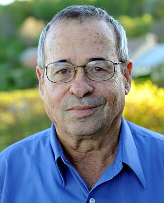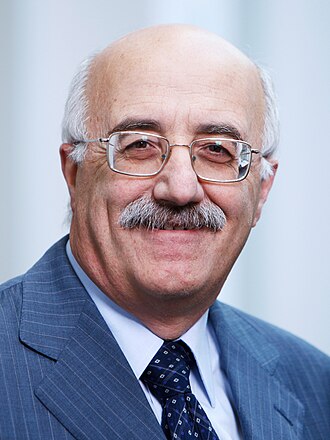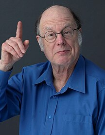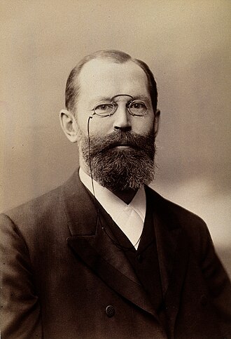
Enciclopédia Histórica Ilustrada • 21 Capítulos • 59 Cientistas com Retrato Oficial VerificadoIllustrated Historical Encyclopedia • 21 Chapters • 59 Scientists with Verified Portraits

The Giants of Quantum Mechanics, Quantum Chemistry & Molecular Modelling Os Gigantes da Mecânica Quântica, Química Quântica e Modelação Molecular

Behind every postulate ($\hat{H}\Psi = E\Psi$), atomic unit ($\text{E}_\text{h}, a_0$), basis set (6-31G*, def2-TZVP), DFT functional (B3LYP, PBE, SCAN), transition-state equation (Eyring, Wigner, Marcus), molecular dynamics integrator, free-energy estimator (BAR), and AI folding network (AlphaFold, Rosetta) stands an extraordinary human story. Meet 59 legendary pioneers across 21 chapters — every single one with their verified portrait photograph, signature equations, impact on Quantum & Computational Chemistry, and a «Funny Story You Will Never Forget 😄»! Por detrás de cada postulado ($\hat{H}\Psi = E\Psi$), unidade atómica ($\text{E}_\text{h}, a_0$), conjunto de base (6-31G*, def2-TZVP), funcional DFT (B3LYP, PBE, SCAN), equação de estado de transição (Eyring, Wigner, Marcus), integrador de dinâmica molecular, estimador de energia livre (BAR) e rede de IA (AlphaFold, Rosetta) está uma história humana extraordinária. Conheça os 59 grandes pioneiros ao longo de 21 capítulos — todos com fotografia individual verificada, equações imortais, impacto na Química Quântica e Computacional e a «Versão Jocosa que Nunca Mais Vais Esquecer 😄»!

⚛️ Parte I • Capítulos 1 a 16 (40 Pioneiros com Fotografia)Part I • Chapters 1 to 16 (40 Pioneers with Photographs)

Os Gigantes da Mecânica Quântica e da Química Quântica (Dos Quanta de Planck à DFT, Espetroscopia e Química Relativista) The Giants of Quantum Mechanics & Quantum Chemistry (From Planck's Quanta to DFT, Spectroscopy & Relativistic Chemistry)

Acompanhe a evolução histórica e humana dos 6 Blocos (Capítulos 1 a 24) do Manual Interativo de Mecânica Quântica: cada entrada liga diretamente os cientistas às equações, conjuntos de base e funcionais que utiliza no ORCA e no Gaussian. Follow the human and historical evolution across all 6 Blocks (Chapters 1 to 24) of the Interactive Quantum Mechanics Textbook: every entry connects the scientists directly to the equations, basis sets, and functionals you run in ORCA and Gaussian.

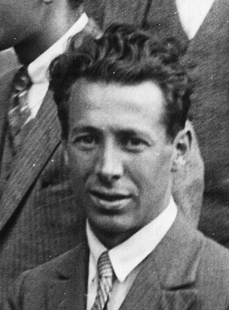
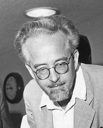
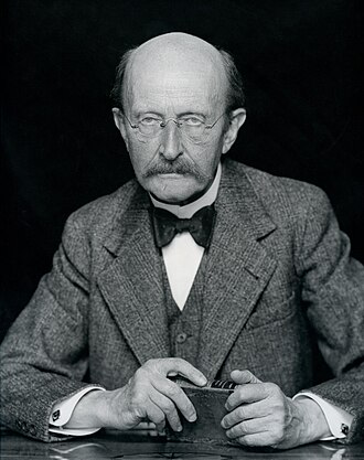
Max Planck
Max Planck 1858–1947
🏆 Nobel Física 1918Nobel Physics 1918 🌐 Wikipedia ↗
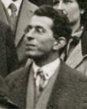
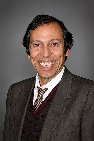
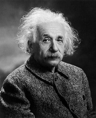
Albert Einstein
Albert Einstein 1879–1955
🏆 Nobel Física 1921Nobel Physics 1921 🌐 Wikipedia ↗
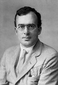
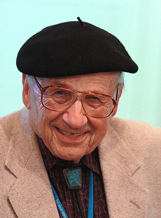
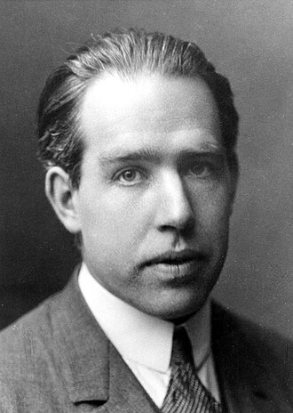
Niels Bohr
Niels Bohr 1885–1962
🏆 Nobel Física 1922Nobel Physics 1922 🌐 Wikipedia ↗
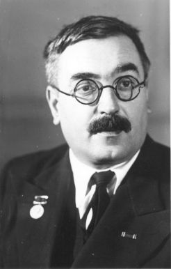
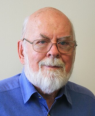
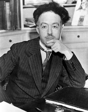
Louis de Broglie
Louis de Broglie 1892–1987
🏆 Nobel Física 1929Nobel Physics 1929 🌐 Wikipedia ↗
QM Block I (Ch. 1) • Light Quanta, Bohr Atom & Wave–Particle DualityQM Bloco I (Cap. 1) • Quanta de Luz, Átomo de Bohr e Dualidade Onda–Partícula Nobel Physics 1918, 1921, 1922 & 1929

1. Max Planck, Albert Einstein, Niels Bohr & Louis de Broglie

Germany, Switzerland, Denmark & France • The Four Founders of the Old Quantum Theory & Matter Waves Alemanha, Suíça, Dinamarca e França • Os Quatro Fundadores da Antiga Teoria Quântica e das Ondas de Matéria

In December 1900, German physicist Max Planck resolved the "Ultraviolet Catastrophe" of blackbody radiation through what he called "an act of desperation": microscopic oscillators inside hot matter cannot exchange energy continuously, but only in discrete packets proportional to $h = 6.62607015\times 10^{-34}\text{ J}\cdot\text{s}$ ($\Delta E = h\nu$). Five years later (1905), Albert Einstein proved that light itself consists of quantized energy packets (photons) that eject electrons from metal surfaces if and only if $h\nu \ge \Phi$ (the Photoelectric Effect, earning him the 1921 Nobel Prize and founding photoelectron spectroscopy PES/XPS). In 1913, Danish physicist Niels Bohr quantized the electron's angular momentum in the Hydrogen atom ($L = n\hbar$), explaining Rydberg's spectral lines, defining the Bohr radius ($a_0 = 0.529177\text{ \AA}$), and rationalizing the Periodic Table. Finally, in his 1924 Paris PhD thesis, French prince Louis de Broglie completed the symmetry: if light waves behave like particles, then every matter particle with momentum $p = mv$ (such as an electron!) behaves as a spatial wave with wavelength $\lambda_{\text{dB}} = h/p$, meaning a stable atomic orbit is simply a standing wave ($2\pi r = n\lambda_{\text{dB}}$)! Em dezembro de 1900, o físico alemão Max Planck resolveu a «Catástrofe do Ultravioleta» da radiação do corpo negro através daquilo a que chamou «um ato de desespero»: os osciladores microscópicos da matéria não trocam energia de forma contínua, mas apenas em pacotes discretos múltiplos de $h = 6.62607015\times 10^{-34}\text{ J}\cdot\text{s}$ ($\Delta E = h\nu$). Cinco anos depois (1905), Albert Einstein provou que a própria luz é constituída por corpúsculos quânticos (fotões) capazes de arrancar eletrões de superfícies metálicas se e só se $h\nu \ge \Phi$ (o Efeito Fotoelétrico, que lhe valeu o Nobel de 1921 e originou a espetroscopia fotoeletrónica PES/XPS). Em 1913, o dinamarquês Niels Bohr quantizou o momento angular do eletrão no átomo de Hidrogénio ($L = n\hbar$), explicando a fórmula espetral de Rydberg, definindo o raio de Bohr ($a_0 = 0.529177\text{ \AA}$) e explicando a arquitetura eletrónica da Tabela Periódica. Finalmente, na sua tese de doutoramento em Paris em 1924, o príncipe francês Louis de Broglie fechou o círculo com uma simetria deslumbrante: se as ondas de luz se comportam como partículas, então todas as partículas com momento linear $p = mv$ (como o eletrão!) têm de se comportar como ondas espaciais de comprimento de onda $\lambda_{\text{dB}} = h/p$, pelo que uma órbita atómica estável é simplesmente uma onda estacionária ($2\pi r = n\lambda_{\text{dB}}$)!

SIGNATURE EQUATIONSEQUAÇÕES IMORTAIS ASSOCIADAS $$\Delta E = h\nu = \hbar\omega, \qquad E_{\text{kin}}^{\max} = h\nu - \Phi, \qquad E_n = -\frac{Z^2}{2n^2}\,\text{E}_{\text{h}}, \qquad \lambda_{\text{dB}} = \frac{h}{p} = \frac{h}{mv}$$
⚛️ Why They Matter in Quantum & Computational ChemistryPorque são importantes em Química Quântica e Computacional

Reduced Planck's constant ($\hbar = h/2\pi$), the Bohr radius ($a_0 = \frac{4\pi\varepsilon_0\hbar^2}{m_e e^2} = 0.529177\text{ \AA}$), and the Hartree energy ($\text{E}_{\text{h}} = \frac{\hbar^2}{m_e a_0^2} = 27.211386\text{ eV} = 627.5095\text{ kcal/mol}$) define the Atomic Units System ($\hbar = m_e = e = 4\pi\varepsilon_0 = 1$) used internally by every quantum chemistry package (ORCA, Gaussian, Q-Chem, Psi4). Meanwhile, the thermal de Broglie wavelength ($\Lambda = h/\sqrt{2\pi m k_B T}$) sets the exact boundary between where classical Molecular Dynamics works (heavy nuclei) and where Quantum Mechanics is mandatory (electrons and proton tunnelling)! A constante de Planck reduzida ($\hbar = h/2\pi$), o raio de Bohr ($a_0 = \frac{4\pi\varepsilon_0\hbar^2}{m_e e^2} = 0.529177\text{ \AA}$) e a energia de Hartree ($\text{E}_{\text{h}} = \frac{\hbar^2}{m_e a_0^2} = 27.211386\text{ eV} = 627.5095\text{ kcal/mol}$) formam o Sistema de Unidades Atómicas ($\hbar = m_e = e = 4\pi\varepsilon_0 = 1$) usado internamente por todos os programas de química quântica (ORCA, Gaussian, Q-Chem, Psi4). E o comprimento de onda térmico de de Broglie ($\Lambda = h/\sqrt{2\pi m k_B T}$) define a fronteira exata entre o mundo onde a Dinâmica Molecular clássica funciona (núcleos pesados) e o mundo onde a Mecânica Quântica é obrigatória (eletrões e efeito de túnel de protões)!

🌍 Why They Matter to the World!Porque são importantes para o Mundo!

Every laser, LED, solar cell, digital camera sensor, UV-Vis/IR spectrophotometer, and transmission electron microscope (Cryo-EM, which uses electron beams with $\lambda_{\text{dB}} \approx 0.02\text{ \AA}$ to image proteins at atomic resolution!) operates on these four equations. Todos os lasers, LEDs, células fotovoltaicas, sensores CCD de câmaras fotográficas, espetrofotómetros UV-Vis/IV e microscópios eletrónicos de transmissão e criomicroscopia (Cryo-EM, que usa feixes de eletrões com $\lambda_{\text{dB}} \approx 0.02\text{ \AA}$ para fotografar proteínas a resolução atómica!) baseiam-se nestas quatro equações.

😄 Funny Version That You Would Never Forget! 😄A Versão Jocosa que Nunca Mais Vais Esquecer! 😄

When young Max Planck told his professor Philipp von Jolly in 1874 that he wanted to study Theoretical Physics, von Jolly solemnly warned him: «Don't do it, young man! Physics is almost completely finished; all that remains is filling in a few sixth-decimal holes!» Planck ignored him and accidentally blew up Classical Physics! And when Louis de Broglie submitted his 1924 PhD thesis at the Sorbonne proposing that electrons are waves, the examining committee was so baffled they mailed a copy to Albert Einstein asking if it was madness or genius. Einstein replied: «He has lifted a corner of the great veil!» — making de Broglie the first scientist in history to win the Nobel Prize directly for his PhD dissertation! Quando o jovem Max Planck disse ao seu professor Philipp von Jolly em 1874 que queria estudar Física Teórica, von Jolly avisou-o solenemente: «Não faça isso, meu jovem! A Física está praticamente terminada; só falta tapar uns pequenos buracos na sexta casa decimal!» Planck ignorou o conselho e destruiu a Física Clássica! Já quando Louis de Broglie entregou a sua tese de doutoramento na Sorbonne em 1924 propondo que os eletrões eram ondas, o júri ficou tão perplexo que enviou uma cópia a Albert Einstein a perguntar se aquilo era loucura ou génio. Einstein respondeu: «Ele levantou uma ponta do grande véu!» — e de Broglie tornou-se o primeiro cientista da história a ganhar o Prémio Nobel diretamente pela sua tese de doutoramento!
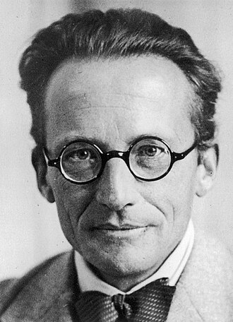
Erwin Schrödinger
Erwin Schrödinger 1887–1961
🏆 Nobel Física 1933Nobel Physics 1933 🌐 Wikipedia ↗
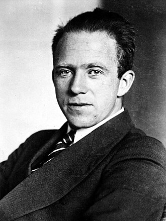
Werner Heisenberg
Werner Heisenberg 1901–1976
🏆 Nobel Física 1932Nobel Physics 1932 🌐 Wikipedia ↗
QM Block I (Ch. 2–4) • Wave Equation, Matrix Mechanics & Uncertainty PrincipleQM Bloco I (Cap. 2–4) • Equação de Onda, Mecânica Matricial e Princípio da Incerteza Nobel Physics 1932 & 1933

2. Erwin Schrödinger (1887–1961) & Werner Heisenberg (1901–1976)

Austria & Germany • Creators of the Wave Equation $\hat{H}\Psi = E\Psi$ & Non-Commuting Matrix Mechanics Áustria e Alemanha • Os Criadores da Equação de Onda $\hat{H}\Psi = E\Psi$ e da Mecânica Matricial Não-Comutativa

In June 1925, retreating to the barren, pollen-free island of Helgoland in the North Sea to survive a severe bout of hay fever, 23-year-old Werner Heisenberg abandoned classical trajectories altogether and formulated Matrix Mechanics in terms of observable transition arrays ($\mathbf{X}\mathbf{P} - \mathbf{P}\mathbf{X} = i\hbar\mathbf{I}$), discovering in 1927 the Uncertainty Principle ($\Delta x\,\Delta p_x \ge \hbar/2$). Months later during Christmas 1925 at an Alpine ski chalet in Arosa (Switzerland), Austrian physicist Erwin Schrödinger followed up on chemist Peter Debye's remark ("If de Broglie's electron is a wave, where is its wave equation?") and derived the time-dependent and time-independent Schrödinger Wave Equation ($\hat{H}\Psi = E\Psi$), proving by March 1926 that differential wave mechanics and Heisenberg's matrix mechanics are mathematically identical! Em junho de 1925, fugindo para a ilha rochosa de Helgoland (no Mar do Norte, sem árvores nem pólen) para sobreviver a uma crise severa de febre dos fenos, Werner Heisenberg (então com apenas 23 anos!) abandonou o conceito clássico de órbita e construiu a Mecânica Matricial baseada apenas em transições observáveis entre estados ($\mathbf{X}\mathbf{P} - \mathbf{P}\mathbf{X} = i\hbar\mathbf{I}$), descobrindo em 1927 o Princípio da Incerteza ($\Delta x\,\Delta p_x \ge \hbar/2$). Poucos meses depois, no Natal de 1925 num chalé alpino em Arosa (Suíça), o físico austríaco Erwin Schrödinger seguiu a sugestão do químico Peter Debye («Se o eletrão de de Broglie é uma onda, onde está a sua equação de onda?») e deduziu a célebre Equação de Schrödinger dependente e independente do tempo ($\hat{H}\Psi = E\Psi$), provando logo em março de 1926 que a sua mecânica ondulatória diferencial e a mecânica matricial de Heisenberg eram matematicamente isomórficas!

SIGNATURE EQUATIONSEQUAÇÕES IMORTAIS ASSOCIADAS $$-\frac{\hbar^2}{2m}\nabla^2\Psi(\mathbf{r}) + V(\mathbf{r})\Psi(\mathbf{r}) = E\Psi(\mathbf{r}), \qquad [\hat{x},\hat{p}_x] = i\hbar, \qquad \sigma_x\,\sigma_{p_x} \ge \frac{\hbar}{2}$$
⚛️ Why They Matter in Quantum & Computational ChemistryPorque são importantes em Química Quântica e Computacional

In Computational Chemistry we use both formulations simultaneously: we write the molecular Hamiltonian as Schrödinger's differential operator ($\hat{H} = -\frac{1}{2}\sum_i\nabla_i^2 - \sum_{i,A}\frac{Z_A}{r_{iA}} + \sum_{i\lt j}\frac{1}{r_{ij}}$), but as soon as we introduce an atomic basis set $\{\phi_\mu\}$, the computer turns Schrödinger's differential equation into Heisenberg's matrix eigenvalue problem ($\mathbf{F}\mathbf{C} = \mathbf{S}\mathbf{C}\boldsymbol{\varepsilon}$)! And Heisenberg's Uncertainty Principle explains why every chemical bond possesses a non-zero Zero-Point Vibrational Energy ($\text{ZPVE} = \frac{1}{2}\sum_k h\nu_k > 0$) even at $T = 0\text{ K}$! Em Química Computacional usamos ambas as formulações em simultâneo: escrevemos o Hamiltoniano molecular como o operador diferencial de Schrödinger ($\hat{H} = -\frac{1}{2}\sum_i\nabla_i^2 - \sum_{i,A}\frac{Z_A}{r_{iA}} + \sum_{i\lt j}\frac{1}{r_{ij}}$), mas assim que introduzimos um conjunto de base atómica $\{\phi_\mu\}$, o computador converte a equação diferencial de Schrödinger na equação matricial de autovalores de Heisenberg ($\mathbf{F}\mathbf{C} = \mathbf{S}\mathbf{C}\boldsymbol{\varepsilon}$)! E o Princípio da Incerteza de Heisenberg explica porque é que todas as ligações químicas têm uma Energia Vibracional de Ponto Zero ($\text{ZPVE} = \frac{1}{2}\sum_k h\nu_k > 0$) mesmo a $T = 0\text{ K}$!

🌍 Why They Matter to the World!Porque são importantes para o Mundo!
Beyond creating the master equation of Quantum Chemistry, Schrödinger published in 1944 in Dublin his landmark book What Is Life?, predicting that chromosomes must be an "aperiodic crystal" encoding a hereditary script — the book that directly inspired James Watson, Francis Crick, and Maurice Wilkins to discover the DNA double helix! Além de criar a equação mestra de toda a Química Quântica, Schrödinger publicou em 1944 em Dublin o pequeno livro What Is Life?, onde previu que os cromossomas tinham de conter um «cristal aperiódico» com um código genético — o livro que levou diretamente James Watson, Francis Crick e Maurice Wilkins a descobrir a dupla hélice do DNA!
😄 Funny Version That You Would Never Forget! 😄A Versão Jocosa que Nunca Mais Vais Esquecer! 😄

Heisenberg almost failed his 1923 PhD oral exam in Munich because experimental physicist Wilhelm Wien asked him the resolving power of an optical microscope and how a lead-acid battery works — and Heisenberg couldn't answer either! Four years later, still haunted by Wien's microscope, Heisenberg imagined a gamma-ray microscope trying to locate an electron and discovered the Uncertainty Principle! Meanwhile, Schrödinger invented his famous dead-and-alive Cat in 1935 not because he liked superposition, but to mock how absurd Bohr and Heisenberg's Copenhagen interpretation sounded when applied to household pets! Heisenberg quase chumbou na prova oral de doutoramento em Munique em 1923 porque o físico experimental Wilhelm Wien lhe perguntou o poder de resolução de um microscópio ótico e o funcionamento de uma bateria de chumbo — e Heisenberg não sabia responder a nenhuma das duas! Quatro anos depois, ainda traumatizado pelo microscópio de Wien, Heisenberg imaginou um microscópio de raios gama a tentar localizar um eletrão e descobriu o Princípio da Incerteza! Já Schrödinger inventou o famoso «Gato de Schrödinger» (vivo e morto ao mesmo tempo dentro de uma caixa) em 1935 não porque gostasse da ideia, mas para ridicularizar a Interpretação de Copenhaga de Bohr e Heisenberg!

Paul A. M. Dirac
Paul A. M. Dirac 1902–1984
🏆 Nobel Física 1933Nobel Physics 1933 🌐 Wikipedia ↗
Wolfgang Pauli
Wolfgang Pauli 1900–1958
🏆 Nobel Física 1945Nobel Physics 1945 🌐 Wikipedia ↗
QM Block I–III (Ch. 2, 7 & 10) • Bra-Ket Notation, Relativistic Equation, Spin & Pauli ExclusionQM Bloco I–III (Cap. 2, 7 & 10) • Notação Bra-Ket, Equação Relativista, Spin e Exclusão de Pauli Nobel Physics 1933 & 1945

3. Paul A. M. Dirac (1902–1984) & Wolfgang Pauli (1900–1958)

UK & Austria/Switzerland • Architects of Bra-Ket Algebra, Relativistic Spin ($s=1/2$) & Fermionic Antisymmetry Reino Unido e Áustria/Suíça • Os Arquitetos da Álgebra Bra-Ket, do Spin Relativista ($s=1/2$) e do Princípio da Antissimetria Fermiónica

In 1925, Austrian physicist Wolfgang Pauli solved the mystery of why all electrons in an atom do not collapse into the lowest $1s$ orbital: he formulated the Pauli Exclusion Principle (no two electrons can share the same four quantum numbers $n, \ell, m_\ell, m_s$), introduced the $2\times 2$ Pauli Spin Matrices ($\boldsymbol{\sigma}_x, \boldsymbol{\sigma}_y, \boldsymbol{\sigma}_z$), and established that the total wave function of any system of electrons (fermions) must be antisymmetric under particle exchange: $\Psi(\dots,\mathbf{x}_i,\dots,\mathbf{x}_j,\dots) = -\Psi(\dots,\mathbf{x}_j,\dots,\mathbf{x}_i,\dots)$. In 1928 at Cambridge, British physicist Paul Dirac invented the universal language of quantum mechanics — Bra-Ket notation ($\langle \phi_i | \hat{O} | \phi_j \rangle$) — and derived the Relativistic Dirac Equation, proving that electron spin $s = 1/2$, the gyromagnetic factor $g_s \approx 2$, spin–orbit coupling, and antimatter (the positron $e^+$, used every day in hospital PET scans!) emerge automatically when quantum mechanics obeys special relativity! Em 1925, o físico austríaco Wolfgang Pauli resolveu o mistério de porque é que todos os eletrões de um átomo não caem para a mesma orbital $1s$: enunciou o Princípio de Exclusão de Pauli (dois eletrões não podem partilhar os mesmos quatro números quânticos $n, \ell, m_\ell, m_s$), introduzindo as Matrizes de Spin de Pauli ($\boldsymbol{\sigma}_x, \boldsymbol{\sigma}_y, \boldsymbol{\sigma}_z$) e formulando que a função de onda total de qualquer sistema de eletrões (fermiões) tem de ser antissimétrica face à troca de quaisquer dois eletrões: $\Psi(\dots,\mathbf{x}_i,\dots,\mathbf{x}_j,\dots) = -\Psi(\dots,\mathbf{x}_j,\dots,\mathbf{x}_i,\dots)$. Em 1928, em Cambridge, o britânico Paul Dirac criou a linguagem universal da mecânica quântica — a notação Bra-Ket ($\langle \phi_i | \hat{O} | \phi_j \rangle$) — e deduziu a Equação Relativista de Dirac para o eletrão, demonstrando que o spin $s = 1/2$, o momento magnético anómalo $g_s \approx 2$, o acoplamento spin-órbita e a própria existência da antimatéria (o positrão $e^+$, usado hoje nos exames hospitalares de PET scan!) decorrem inevitavelmente da união entre a Mecânica Quântica e a Relatividade Restrita!

SIGNATURE EQUATIONSEQUAÇÕES IMORTAIS ASSOCIADAS $$\Psi(\mathbf{x}_1,\mathbf{x}_2) = -\Psi(\mathbf{x}_2,\mathbf{x}_1), \qquad \langle \phi_\mu | \hat{H} | \phi_\nu \rangle = H_{\mu\nu}, \qquad (i\hbar\gamma^\mu\partial_\mu - m_e c)\psi = 0$$
⚛️ Why They Matter in Quantum & Computational ChemistryPorque são importantes em Química Quântica e Computacional

Without Pauli's Exclusion Principle there would be no Periodic Table, no chemical valence, and no steric repulsion (the short-range $A/r^{12}$ wall in Molecular Dynamics force fields is physically Pauli exchange repulsion when two closed-shell electron clouds overlap!). And in 1929, Paul Dirac wrote the founding charter of Computational Chemistry: «The underlying physical laws necessary for the mathematical theory of a large part of physics and the whole of chemistry are thus completely known, and the difficulty is only that the exact application of these laws leads to equations much too complicated to be soluble. It therefore becomes desirable that approximate practical methods of applying quantum mechanics should be developed.» Sem o Princípio de Exclusão de Pauli não existiria Tabela Periódica, nem valência química, nem impedimento estérico (a repulsão de curto alcance $A/r^{12}$ nos campos de forças de Dinâmica Molecular é, na verdade, repulsão de troca de Pauli quando duas nuvens eletrónicas de camada fechada se sobrepõem!). E em 1929, Paul Dirac escreveu a frase que fundou a Química Computacional: «As leis físicas necessárias para a teoria matemática de toda a Química são assim completamente conhecidas, e a única dificuldade é que as equações são demasiado complicadas para serem resolvidas exatamente — tornando-se desejável desenvolver métodos práticos aproximados.»

🌍 Why They Matter to the World!Porque são importantes para o Mundo!

Pauli's Exclusion Principle keeps solid matter (and white dwarf stars!) from collapsing, while Dirac's equation explains heavy-element chemistry (gold, platinum, mercury, lanthanides) and Positron Emission Tomography (PET) in cancer imaging. O Princípio de Pauli impede a matéria sólida (e as estrelas anãs brancas!) de colapsar sobre si própria, enquanto a equação de Dirac explica a química dos metais pesados (ouro, platina, mercúrio, lantanídeos) e a Tomografia por Emissão de Positrões (PET) no diagnóstico oncológico.

😄 Funny Version That You Would Never Forget! 😄A Versão Jocosa que Nunca Mais Vais Esquecer! 😄

Wolfgang Pauli was such a ruthless critic of sloppy theoretical papers that he coined the ultimate scientific insult after reading a muddled manuscript: «This isn't right. It's not even wrong!» («Das ist nicht einmal falsch!») Experimentalists also feared the legendary "Pauli Effect": whenever the pure theorist Pauli walked into a laboratory, vacuum equipment would mysteriously shatter! Meanwhile, Paul Dirac was so famously silent at Cambridge that colleagues defined the unit «1 Dirac = 1 word per hour». Wolfgang Pauli era um crítico tão implacável de artigos científicos mal pensados que cunhou o insulto supremo da Física Teórica ao ler um artigo confuso: «Isto não está sequer errado!» («Das ist nicht einmal falsch!») Além disso, era lendário o «Efeito Pauli»: sempre que o teórico Pauli entrava num laboratório experimental, algum aparelho de vácuo explodia misteriosamente! Já Paul Dirac era tão silencioso em Cambridge que os estudantes definiram a unidade «1 Dirac = 1 palavra por hora». Quando um jornalista americano lhe pediu para resumir a filosofia da sua vida numa frase, Dirac respondeu: «Na escola ensinaram-me a nunca começar uma frase sem saber como a acabar.»

Max Born
Max Born 1882–1970
🏆 Nobel Física 1954Nobel Physics 1954 🌐 Wikipedia ↗
J. Robert Oppenheimer
J. Robert Oppenheimer 1904–1967
🏆 Aprox. Born–Oppenheimer 1927Born–Oppenheimer 1927 🌐 Wikipedia ↗
QM Block I & III (Ch. 3 & 11) • Born Rule $|\Psi|^2$ & Potential Energy Surface (PES)QM Bloco I & III (Cap. 3 & 11) • Regra de Born $|\Psi|^2$ e Superfície de Energia Potencial (PES) 1926–1927 • Nobel Physics 1954

4. Max Born (1882–1970) & J. Robert Oppenheimer (1904–1967)

Germany & USA • Creators of the Probabilistic Wave Function & the Potential Energy Surface $U(\mathbf{R})$ Alemanha e EUA • Os Criadores da Interpretação Probabilística e da Superfície de Energia Potencial $U(\mathbf{R})$

When Schrödinger wrote $\hat{H}\Psi = E\Psi$ in 1926, nobody knew what $\Psi$ physically meant: Schrödinger initially thought the electron's charge was literally smeared out in space. In June 1926, Göttingen professor Max Born discovered the truth: $\Psi(\mathbf{r})$ is a complex probability amplitude whose squared modulus, $\rho_{\text{prob}}(\mathbf{r}) = |\Psi(\mathbf{r})|^2$, gives the physical probability density of finding the particle in volume element $d\mathbf{r}$! The following year (1927), Born and his 22-year-old American PhD student J. Robert Oppenheimer published in Annalen der Physik the Born–Oppenheimer Approximation: because the electron-to-nuclear mass ratio is tiny ($\kappa = (m_e/M_A)^{1/4} \ll 1$, as even a single proton is $1,836\times$ heavier than an electron), electrons move thousands of times faster and adjust instantaneously to any nuclear geometry $\mathbf{R}$, factoring $\Psi_{\text{total}}(\mathbf{r},\mathbf{R}) \approx \Psi_{\text{elec}}(\mathbf{r};\mathbf{R})\,\chi_{\text{nucl}}(\mathbf{R})$! Quando Schrödinger escreveu $\hat{H}\Psi = E\Psi$ em 1926, ninguém sabia o que significava fisicamente a função de onda $\Psi$: Schrödinger pensava que a carga do eletrão estava fisicamente espalhada pelo espaço. Em junho de 1926, o professor de Göttingen Max Born descobriu a verdade: $\Psi(\mathbf{r})$ é uma amplitude complexa de probabilidade cujo módulo ao quadrado, $\rho_{\text{prob}}(\mathbf{r}) = |\Psi(\mathbf{r})|^2$, fornece a densidade de probabilidade de encontrar a partícula no elemento de volume $d\mathbf{r}$! No ano seguinte (1927), Born e o seu brilhante estudante de doutoramento americano de 22 anos, J. Robert Oppenheimer, publicaram nos Annalen der Physik a Aproximação de Born–Oppenheimer: como a razão de massas eletrão/núcleo é pequeníssima ($\kappa = (m_e/M_A)^{1/4} \ll 1$, pois o protão é $1\,836\times$ mais pesado do que o eletrão), os eletrões movem-se milhares de vezes mais depressa e ajustam-se instantaneamente a qualquer posição nuclear $\mathbf{R}$, permitindo fatorizar $\Psi_{\text{total}}(\mathbf{r},\mathbf{R}) \approx \Psi_{\text{ele}}(\mathbf{r};\mathbf{R})\,\chi_{\text{nuc}}(\mathbf{R})$!

SIGNATURE EQUATIONSEQUAÇÕES IMORTAIS ASSOCIADAS $$P(\mathbf{r}\in d\mathbf{r}) = |\Psi(\mathbf{r})|^2\,d\mathbf{r}, \qquad \hat{H}_{\text{elec}}(\mathbf{r};\mathbf{R})\Psi_{\text{elec}}(\mathbf{r};\mathbf{R}) = E_{\text{elec}}(\mathbf{R})\Psi_{\text{elec}}(\mathbf{r};\mathbf{R}), \qquad U_{\text{PES}}(\mathbf{R}) = E_{\text{elec}}(\mathbf{R}) + \sum_{A
⚛️ Why They Matter in Quantum & Computational ChemistryPorque são importantes em Química Quântica e Computacional

The Born–Oppenheimer Approximation is the bedrock of all Structural Chemistry and Molecular Modelling: without it, the very concepts of molecular geometry (bond lengths and angles), Potential Energy Surfaces $U_{\text{PES}}(\mathbf{R})$, transition states ($\text{TS}^\ddagger$), and Molecular Dynamics Force Fields would not exist! Moreover, in 1920 Max Born also derived the Born Continuum Ion Solvation Model ($\Delta G_{\text{solv}} = -\frac{q^2}{8\pi\varepsilon_0 r_0}(1 - 1/\varepsilon_r)$), the ancestor of all modern PCM, COSMO, SMD, and MM-GBSA implicit solvent models! A Aproximação de Born–Oppenheimer é o alicerce de toda a Química Estrutural e de toda a Modelação Molecular: sem ela, não existiria o conceito de geometria molecular (comprimentos e ângulos de ligação), nem Superfície de Energia Potencial $U_{\text{PES}}(\mathbf{R})$, nem estados de transição ($\text{TS}^\ddagger$), nem Campos de Forças de Dinâmica Molecular! E em 1920, Max Born também criou o Modelo de Solvatação Iónica Contínua de Born ($\Delta G_{\text{solv}} = -\frac{q^2}{8\pi\varepsilon_0 r_0}(1 - 1/\varepsilon_r)$), a equação avó de todos os modelos modernos PCM, COSMO, SMD e MM-GBSA!

🌍 Why They Matter to the World!Porque são importantes para o Mundo!

Allows chemists and biologists to picture chemical reactions and protein folding as journeys across a 3D mountain landscape of valleys (reactants, products, conformers) and mountain passes (transition states). Permite visualizar reações químicas e o folding de proteínas como caminhadas sobre uma paisagem montanhosa 3D de vales (reagentes, produtos, confórmeros) e passos de montanha (estados de transição).

😄 Funny Version That You Would Never Forget! 😄A Versão Jocosa que Nunca Mais Vais Esquecer! 😄

Max Born put the $|\Psi|^2$ rule — one of the deepest postulates in the history of science — in a tiny footnote of his 1926 paper because in his first draft he had written $|\Psi|$ and fixed it to $|\Psi|^2$ in the galley proofs! That single footnote won him the 1954 Nobel Prize! Meanwhile in Göttingen, young Robert Oppenheimer interrupted seminar speakers so relentlessly to jump to the blackboard and finish their equations that his fellow PhD students presented Max Born with a formal petition on parchment threatening to boycott seminars unless Born made Oppenheimer stop talking! Max Born colocou a regra $|\Psi|^2$ — um dos postulados mais profundos da história da ciência — numa pequena nota de rodapé do seu artigo de 1926 porque na primeira versão tinha escrito $|\Psi|$ em vez de $|\Psi|^2$ e corrigiu nas provas tipográficas! Essa nota de rodapé valeu-lhe o Nobel da Física de 1954! E em Göttingen, o jovem Robert Oppenheimer interrompia de tal maneira todos os oradores nos seminários para ir ao quadro acabar as deduções deles que os colegas de doutoramento organizaram uma petição em pergaminho assinada ameaçando boicotar as aulas se Max Born não mandasse calar o Oppenheimer!

Walter Heitler
Walter Heitler 1904–1981
🏆 Medalha Max Planck 1968Max Planck Medal 1968 🌐 Wikipedia ↗
Fritz London
Fritz London 1900–1954
🏆 Medalha Lorentz 1953Lorentz Medal 1953 🌐 Wikipedia ↗
QM Block III & IV (Ch. 12 & 16) • The 1st Quantum Chemical Bond ($\text{H}_2$, 1927) & London Dispersion ($-C_6/R^6$)QM Bloco III & IV (Cap. 12 & 16) • A 1.ª Ligação Química Quântica ($\text{H}_2$, 1927) e Dispersão de London ($-C_6/R^6$) 1927 & 1930 • Birth of Quantum Chemistry

5. Walter Heitler (1904–1981) & Fritz London (1900–1954)

Germany • Authors of the 1927 Paper Explaining the Covalent Bond & the 1930 Theory of London Dispersion Forces Alemanha • Os Autores do Artigo de 1927 que Explicou a Ligação Covalente e do Artigo de 1930 das Forças de Dispersão de van der Waals

For over a century after Berzelius and Gilbert N. Lewis, nobody could physically explain how two neutral Hydrogen atoms ($\text{H}\cdot + \cdot\text{H}$) share an electron pair to form a strong covalent bond ($\text{H}-\text{H}$, $D_e = 4.75\text{ eV} = 458\text{ kJ/mol}$), since classically two negative electrons repel! In June 1927 in Zurich, two young German postdocs, Walter Heitler and Fritz London, applied Schrödinger's brand-new wave equation to the $\text{H}_2$ molecule and uncovered the secret: because the two electrons are indistinguishable, the symmetric spatial wave function $\Psi_+(1,2) \propto \phi_A(1)\phi_B(2) + \phi_B(1)\phi_A(2)$ generates a purely quantum constructive interference and exchange integral ($K_{AB}$) that piles up electron density right between the two positive nuclei, gluing them together! Three years later (1930), Fritz London applied second-order perturbation theory to two neutral atoms at long range and proved that correlated quantum fluctuations of electron clouds create instantaneous induced dipoles that always attract via the universal $V_{\text{disp}}(R) = -C_6 / R^6$ law (London Dispersion Forces)! Durante mais de um século após Berzelius e Gilbert N. Lewis, ninguém sabia explicar fisicamente como é que dois átomos neutros de Hidrogénio ($\text{H}\cdot + \cdot\text{H}$) partilham um par de eletrões para formar uma ligação covalente forte ($\text{H}-\text{H}$, $D_e = 4.75\text{ eV} = 458\text{ kJ/mol}$), já que classicamente dois eletrões negativos se repelem! Em junho de 1927, em Zurique, dois jovens pós-doutorandos alemães, Walter Heitler e Fritz London, aplicaram a equação de Schrödinger de 1926 à molécula de $\text{H}_2$ e descobriram o segredo: como os dois eletrões são indistinguíveis, a função de onda espacial simétrica $\Psi_+(1,2) \propto \phi_A(1)\phi_B(2) + \phi_B(1)\phi_A(2)$ cria um termo puramente quântico de interferência construtiva e troca ($K_{AB}$) que acumula densidade eletrónica exatamente a meio caminho entre os dois núcleos positivos, colando-os! Três anos depois (1930), Fritz London aplicou a teoria das perturbações de 2.ª ordem a dois átomos neutros de gás nobre a longa distância e provou que as flutuações quânticas correlacionadas das nuvens eletrónicas criam dipolos instantâneos induzidos que se atraem sempre com a lei universal $V_{\text{disp}}(R) = -C_6 / R^6$ (Forças de Dispersão de London)!

SIGNATURE EQUATIONSEQUAÇÕES IMORTAIS ASSOCIADAS $$\Psi_{\text{VB}}^{\text{HL}}(1,2) = \frac{\phi_A(1)\phi_B(2) + \phi_B(1)\phi_A(2)}{\sqrt{2(1+S_{AB}^2)}}, \qquad E_{\text{disp}}^{\text{London}}(R) = -\frac{3}{2}\frac{I_A I_B}{I_A + I_B}\frac{\alpha_A\alpha_B}{(4\pi\varepsilon_0)^2 R^6} = -\frac{C_6}{R^6}$$
⚛️ Why They Matter in Quantum & Computational ChemistryPorque são importantes em Química Quântica e Computacional

Heitler & London's paper of June 30, 1927 marks the official birth date of Quantum Chemistry! And Fritz London's 1930 $-C_6/R^6$ law is the attractive term of every Lennard-Jones 12-6 potential in Molecular Dynamics ($4\varepsilon[(\sigma/r)^{12} - (\sigma/r)^6]$) as well as the physical foundation of Stefan Grimme's D3(BJ) and D4 dispersion corrections in modern DFT calculations (Ch. 16)! O artigo de Heitler & London de 30 de junho de 1927 marca a data de nascimento oficial da Química Quântica! E a lei $-C_6/R^6$ de Fritz London (1930) é o termo atrativo de todos os potenciais de Lennard-Jones 12-6 em Dinâmica Molecular ($4\varepsilon[(\sigma/r)^{12} - (\sigma/r)^6]$) e a base física das correções de dispersão D3(BJ) e D4 de Stefan Grimme em todos os cálculos DFT modernos (Cap. 16)!

🌍 Why They Matter to the World!Porque são importantes para o Mundo!

London dispersion forces explain why gases condense into liquids, why the DNA double helix is stabilized by $\pi$-$\pi$ base stacking, how hydrophobic drugs bind to protein pockets, and how geckos walk upside down across polished glass ceilings! As forças de dispersão de London explicam porque é que o azoto e o hélio podem ser liquefeitos, porque é que a dupla hélice do DNA é estabilizada pelo empilhamento aromático ($\pi$-$\pi$ stacking) das bases azotadas, como é que os fármacos hidrofóbicos se ligam às proteínas e como é que as osgas (geckos) caminham de cabeça para baixo num teto de vidro polido!

😄 Funny Version That You Would Never Forget! 😄A Versão Jocosa que Nunca Mais Vais Esquecer! 😄

How did Heitler and London discover the quantum covalent bond in Zurich in a single spring afternoon in 1927? They had computed the classical electrostatic overlap between two hydrogen atoms (which gave barely any binding!) and went to bed disappointed. The next morning they remembered Heisenberg's exchange symmetry for indistinguishable electrons, wrote down the cross term $\phi_A(1)\phi_B(2) + \phi_B(1)\phi_A(2)$ over lunch, and by late afternoon realized they had just explained chemical bonding across the entire Periodic Table! Como é que Heitler e London descobriram a ligação covalente quântica em Zurique numa única tarde de primavera de 1927? Tinham calculado o integral eletrostático clássico entre dois átomos de hidrogénio (que dava quase zero!) e foram dormir desanimados. Na manhã seguinte, lembraram-se da simetria de Heisenberg para eletrões indistinguíveis, somaram o termo cruzado $\phi_A(1)\phi_B(2) + \phi_B(1)\phi_A(2)$ à hora de almoço e descobriram ao final da tarde que tinham acabado de explicar toda a ligação química da Tabela Periódica!

Douglas R. Hartree
Douglas R. Hartree 1897–1958
🏆 Unidade Hartree (Eh)Hartree Unit (Eh) 🌐 Wikipedia ↗
Vladimir A. Fock
Vladimir A. Fock 1898–1974
🏆 Operador de FockFock Operator 🌐 Wikipedia ↗
John C. Slater
John C. Slater 1900–1976
🏆 Medalha Nacional CiênciaNational Medal of Science 🌐 Wikipedia ↗
QM Block III & IV (Ch. 10, 13 & 14) • Self-Consistent Field (SCF), Slater Determinants & Exact ExchangeQM Bloco III & IV (Cap. 10, 13 & 14) • Campo Autoconsistente (SCF), Determinantes de Slater e Troca Exata 1928 – 1930 • Foundation of Ab Initio Theory

6. Douglas Hartree (1897–1958), Vladimir Fock (1898–1974) & John C. Slater (1900–1976)

UK, USSR & USA • Creators of the Hartree–Fock SCF Method, Slater Determinants & Slater-Type Orbitals Reino Unido, URSS e EUA • Os Criadores do Método de Hartree–Fock, do Determinante de Slater e das Orbitais STO

How do you solve the Schrödinger equation for an atom or molecule with $N$ mutually repelling electrons coupled by the singular operator $1/r_{ij}$? In 1928, British mathematician Douglas Hartree proposed the Self-Consistent Field (SCF) method: replace instantaneous two-electron repulsion with an iterative average electrostatic field generated by the other $N-1$ electron clouds. In 1929–1930, MIT physicist John C. Slater proved that Pauli's Antisymmetry Principle is satisfied automatically for any $N$-electron system by writing the wave function as a single Slater Determinant of spin-orbitals (and also introduced Slater-Type Orbitals, STO, $r^{n-1}e^{-\zeta r}$, and Slater's nuclear shielding rules!). Simultaneously in 1930, Soviet physicist Vladimir Fock (and independently Slater) applied the variational principle to a Slater Determinant, unveiling the purely quantum Non-Local Exchange Operator ($\hat{K}_j$) and establishing the Hartree–Fock Equations ($\hat{f}\chi_i = \varepsilon_i\chi_i$)! Como resolver a equação de Schrödinger para um átomo ou molécula com $N$ eletrões que se repelem todos mutuamente através do operador singular $1/r_{ij}$? Em 1928, o matemático britânico Douglas Hartree propôs o Método do Campo Autoconsistente (SCF): substituir a repulsão instantânea por um campo eletrostático médio iterativo gerado pelas nuvens dos outros $N-1$ eletrões. Em 1929–1930, o físico americano do MIT John C. Slater provou que o Princípio de Antissimetria de Pauli é automaticamente satisfeito para qualquer número $N$ de eletrões escrevendo a função de onda como um único Determinante de Slater de spin-orbitais (e introduziu ainda as Orbitais do Tipo de Slater, STO, $r^{n-1}e^{-\zeta r}$, e as regras de blindagem nuclear de Slater!). Em simultâneo (1930), o físico soviético Vladimir Fock (e independentemente Slater) aplicou o princípio variacional ao Determinante de Slater, fazendo emergir o Operador de Troca Não-Local ($\hat{K}_j$) e criando as Equações Integrodiferenciais de Hartree–Fock ($\hat{f}\chi_i = \varepsilon_i\chi_i$)!

SIGNATURE EQUATIONSEQUAÇÕES IMORTAIS ASSOCIADAS $$\Psi_{\text{SD}} = \frac{1}{\sqrt{N!}}\det|\chi_1\chi_2\cdots\chi_N|, \qquad \hat{f}(1)\chi_i(1) = \left[\hat{h}(1) + \sum_{j=1}^{N}\left(\hat{J}_j(1) - \hat{K}_j(1)\right)\right]\chi_i(1) = \varepsilon_i\chi_i(1)$$
⚛️ Why They Matter in Quantum & Computational ChemistryPorque são importantes em Química Quântica e Computacional

The Hartree–Fock (HF) method is the cornerstone of electronic structure theory: it recovers ~99% of the total electronic energy, cancels each electron's spurious self-interaction exactly ($J_{ii} - K_{ii} = 0$, which is why Rung-4 hybrid DFT functionals must mix in a fraction $a_0$ of exact HF exchange!), and provides the reference determinant $\Phi_0$ for all correlated MP2, CCSD(T), and CASPT2 methods! O método de Hartree–Fock (HF) é a pedra angular de toda a estrutura eletrónica: recupera ~99% da energia eletrónica total, cancela exatamente a auto-interação espúria de cada eletrão consigo mesmo ($J_{ii} - K_{ii} = 0$, razão pela qual os funcionais DFT híbridos precisam de misturar uma fração $a_0$ de troca exata de Hartree–Fock no Degrau 4 da Escada de Jacob!) e fornece o determinante de referência $\Phi_0$ para todos os métodos correlacionados MP2, CCSD(T) e CASPT2!

🌍 Why They Matter to the World!Porque são importantes para o Mundo!

Gave rigorous mathematical meaning to individual orbitals ($\chi_i$) and orbital energies ($\varepsilon_i$) in many-electron atoms and molecules, underpinning modern organic, inorganic, and spectroscopic chemistry. Deu existência matemática rigorosa ao conceito de orbital individual ($\chi_i$) e de energia orbital ($\varepsilon_i$) num sistema multieletrónico, sustentando toda a química orgânica, inorgânica e espetroscópica moderna.

😄 Funny Version That You Would Never Forget! 😄A Versão Jocosa que Nunca Mais Vais Esquecer! 😄

How did Douglas Hartree converge Self-Consistent Field (SCF) cycles in 1928 before electronic computers existed? He recruited his retired father, William Hartree, who sat at the kitchen table with a hand-cranked mechanical calculator for 15 years numerically integrating atomic orbitals by hand! And in 1934, Douglas Hartree and his student Arthur Porter built an analog Differential Analyzer at Manchester University entirely out of children's Meccano construction toys (costing just £20!) that solved atomic Hartree–Fock wave functions to within 2% accuracy! Como é que Douglas Hartree convergia ciclos de Campo Autoconsistente (SCF) em 1928 antes de existirem computadores eletrónicos? Recrutou o próprio pai reformado, William Hartree, que passou 15 anos sentado à mesa da cozinha com uma calculadora mecânica a manivela a integrar numericamente orbitais atómicas à mão! E em 1934, Douglas Hartree e o seu aluno Arthur Porter construíram na Universidade de Manchester um computador analógico diferencial feito inteiramente com peças de brinquedo Meccano de criança (custando apenas 20 libras!) que resolvia funções de onda atómicas de Hartree–Fock com 98% de exatidão!

Linus C. Pauling
Linus C. Pauling 1901–1994
🏆 Nobel Química 1954 & Paz 1962Nobel Chem 1954 & Peace 1962 🌐 Wikipedia ↗
Robert S. Mulliken
Robert S. Mulliken 1896–1986
🏆 Nobel Química 1966Nobel Chemistry 1966 🌐 Wikipedia ↗
Friedrich Hund
Friedrich Hund 1896–1997
🏆 Medalha Max Planck 1943Max Planck Medal 1943 🌐 Wikipedia ↗
QM Block II, III & V (Ch. 8, 12 & 19) • Valence Bond (VB) vs. Molecular Orbitals (LCAO-MO) & Hund's RulesQM Bloco II, III & V (Cap. 8, 12 & 19) • Ligação de Valência (VB) vs. Orbitais Moleculares (LCAO-MO) e Regras de Hund Nobel Chemistry 1954 & 1966 • Peace 1962

7. Linus Pauling (1901–1994), Robert S. Mulliken (1896–1986) & Friedrich Hund (1896–1997)

USA & Germany • Architects of $sp^3/sp^2/sp$ Hybridization, Delocalized Molecular Orbitals, Hund's Rules & Quantum Tunnelling EUA e Alemanha • Os Arquitetos da Hibridação $sp^3/sp^2/sp$, das Orbitais Moleculares Deslocalizadas, das Regras de Hund e do Efeito de Túnel

Between 1927 and 1935, the two great rival (and complementary!) schools of molecular electronic structure were born. At Caltech, Linus Pauling expanded Heitler–London theory into Valence Bond (VB) Theory, introducing orbital hybridization ($sp^3$ tetrahedral at $109.5^\circ$, $sp^2$ trigonal, and $sp$ linear), resonance, the electronegativity scale, the protein $\alpha$-helix and $\beta$-sheet, and the foundational principle of enzyme catalysis (enzymes selectively stabilize the Transition State $\text{TS}^\ddagger$!). Simultaneously at Chicago and Göttingen/Leipzig, Robert S. Mulliken ("Mr. Molecule", who coined the word "orbital" in 1932!) and Friedrich Hund created Molecular Orbital (MO) Theory via Linear Combination of Atomic Orbitals (LCAO-MO, $\psi_i = \sum_\mu c_{\mu i}\phi_\mu$), showing that electrons belong to the entire molecule and immediately explaining why the oxygen we breathe ($\text{O}_2$, triplet ground state $^3\Sigma_g^-$ with two unpaired electrons in degenerate $\pi_g^*$ orbitals!) is paramagnetic via Hund's Maximum Multiplicity Rule! Moreover, in 1927 Friedrich Hund was the first physicist in history to discover Quantum Tunnelling by calculating the double-well umbrella inversion of the ammonia ($\text{NH}_3$) molecule! Entre 1927 e 1935 nasceram as duas grandes escolas rivais (e complementares!) da estrutura eletrónica molecular. No Caltech, Linus Pauling generalizou a teoria de Heitler–London na Teoria da Ligação de Valência (VB), introduzindo a hibridação orbital ($sp^3$ tetraédrica de $109.5^\circ$, $sp^2$ trigonal e $sp$ linear), a ressonância, a escala de eletronegatividade, a hélice $\alpha$ e a folha $\beta$ das proteínas, e o princípio fundador da catálise enzimática (as enzimas estabilizam seletivamente o Estado de Transição $\text{TS}^\ddagger$!). Em simultâneo, na Universidade de Chicago e em Göttingen/Leipzig, Robert S. Mulliken («Mr. Molecule», que inventou a própria palavra «orbital» em 1932!) e Friedrich Hund criaram a Teoria das Orbitais Moleculares (MO) via Combinação Linear de Orbitais Atómicas (LCAO-MO, $\psi_i = \sum_\mu c_{\mu i}\phi_\mu$), mostrando que os eletrões pertencem à molécula inteira e explicando imediatamente porque é que o oxigénio que respiramos ($\text{O}_2$, estado fundamental tripleto $^3\Sigma_g^-$ com dois eletrões desemparelhados nas orbitais $\pi_g^*$ degeneradas!) é paramagnético pelas Regras de Multiplicidade Máxima de Hund! Além disso, em 1927, Friedrich Hund foi o primeiro físico da história a descobrir o Efeito de Túnel Quântico ao calcular a inversão piramidal de barreira dupla da molécula de amoníaco ($\text{NH}_3$)!

SIGNATURE EQUATIONSEQUAÇÕES IMORTAIS ASSOCIADAS $$\psi_i(\mathbf{r}) = \sum_{\mu=1}^{K} c_{\mu i}\,\phi_\mu(\mathbf{r}), \qquad N_{\text{ele}} = \operatorname{Tr}(\mathbf{P}\mathbf{S}), \qquad q_A^{\text{Mulliken}} = Z_A - \sum_{\mu\in A}(\mathbf{P}\mathbf{S})_{\mu\mu}$$
⚛️ Why They Matter in Quantum & Computational ChemistryPorque são importantes em Química Quântica e Computacional

Every modern electronic structure program (ORCA, Gaussian, Molpro) constructs Kohn–Sham and Hartree–Fock orbitals using the Hund–Mulliken LCAO-MO expansion ($\psi_i = \sum_\mu c_{\mu i}\phi_\mu$) and prints Mulliken Population Analysis (1955) ($\mathbf{P}\mathbf{S}$) at the end of the SCF cycle. Meanwhile, Hund's Rules govern the high-spin vs. low-spin states of every bioinorganic metal center (such as the $\text{Fe}^{2+}$ Heme group in hemoglobin and cytochrome P450)! Todos os programas modernos de estrutura eletrónica (ORCA, Gaussian, Molpro) constroem as orbitais de Kohn–Sham e de Hartree–Fock usando a expansão LCAO-MO de Hund–Mulliken ($\psi_i = \sum_\mu c_{\mu i}\phi_\mu$) e imprimem no final a Análise Populacional de Mulliken (1955) ($\mathbf{P}\mathbf{S}$). E as Regras de Hund governam os estados de alto spin vs. baixo spin de todos os centros metálicos bioinorgânicos (como o grupo Heme $\text{Fe}^{2+}$ da hemoglobina e dos citocromos P450)!

🌍 Why They Matter to the World!Porque são importantes para o Mundo!

Pauling remains the only person in history awarded two unshared Nobel Prizes (Chemistry 1954 and Peace 1962), while Friedrich Hund lived to age 101, mentoring generations of 20th-century quantum scientists! Pauling é a única pessoa na história mundial galardoada com dois Prémios Nobel individuais não partilhados (Química 1954 e Paz 1962), e Friedrich Hund viveu até aos 101 anos, tendo ensinado quase todas as gerações de físicos alemães do século XX!

😄 Funny Version That You Would Never Forget! 😄A Versão Jocosa que Nunca Mais Vais Esquecer! 😄

How did Linus Pauling discover the protein $\alpha$-helix in 1948? Stuck in bed in Oxford with a bad cold and bored of detective novels, he took a strip of paper, drew a polypeptide backbone keeping the peptide bond planar (as his own resonance theory required!), and folded the paper like origami until the $\text{N–H}\cdots\text{O=C}$ hydrogen bonds clicked into place every $3.6$ residues! Meanwhile, Robert Mulliken famously quipped: «The more accurate the calculations become, the more the concepts of chemistry tend to vanish into thin air!» Como é que Linus Pauling descobriu a hélice $\alpha$ das proteínas em 1948? Estava de cama em Oxford com uma gripe forte, cansou-se de ler romances policiais, pediu papel, lápis e uma régua, desenhou uma cadeia polipeptídica respeitando a planaridade da ligação peptídica que ele próprio tinha previsto por ressonância, e dobrou a tira de papel como um origami até as pontes de hidrogénio $\text{N–H}\cdots\text{O=C}$ encaixarem a cada $3.6$ resíduos! Já Robert Mulliken resumiu o dilema da Química Computacional numa frase imortal: «Quanto mais exatos se tornam os nossos cálculos quânticos, mais os conceitos tradicionais da química parecem evaporar-se no ar!»

Erich Hückel
Erich Hückel 1896–1980
🏆 Regra 4n+2 (1931)4n+2 Rule (1931) 🌐 Wikipedia ↗
Charles A. Coulson
Charles A. Coulson 1910–1974
🏆 Medalha Davy 1970Davy Medal 1970 🌐 Wikipedia ↗
Michael J. S. Dewar
Michael J. S. Dewar 1918–1997
🏆 Medalha Davy 1982Davy Medal 1982 🌐 Wikipedia ↗
QM Block II & III (Ch. 5 & 12) • Conjugated $\pi$ Systems, $4n+2$ Aromaticity & Semi-Empirical MethodsQM Bloco II & III (Cap. 5 & 12) • Sistemas $\pi$ Conjugados, Aromaticidade $4n+2$ e Métodos Semi-Empíricos 1931 – 1985 • Organic Quantum Chemistry

8. Erich Hückel (1896–1980), Charles A. Coulson (1910–1974) & Michael J. S. Dewar (1918–1997)

Germany & UK/USA • Pioneers of Hückel Theory, the $4n+2$ Aromaticity Rule, Fractional Bond Orders & Semi-Empirical Methods Alemanha e Reino Unido/EUA • Os Pioneiros da Teoria de Hückel, da Regra $4n+2$ da Aromaticidade, das Ordens de Ligação Fracionárias e dos Métodos Semi-Empíricos

After co-creating with Peter Debye the famous Debye–Hückel theory of electrolyte solutions (1923), German physicist Erich Hückel tackled organic chemistry's greatest puzzle since Kekulé (1865): why is benzene ($\text{C}_6\text{H}_6$, with 6 $\pi$ electrons) extraordinarily stable and aromatic, whereas cyclobutadiene ($\text{C}_4\text{H}_4$, 4 $\pi$ electrons) and cyclooctatetraene ($\text{C}_8\text{H}_8$, 8 $\pi$ electrons) are not? In 1931, Hückel separated $\sigma$ and $\pi$ frameworks ($\mathbf{H}_\pi\mathbf{c} = E\mathbf{c}$, parameterized by Coulomb integral $\alpha$ and resonance integral $\beta \lt 0$) and derived the immortal Hückel $4n + 2$ Rule for aromatic rings! At Oxford, British mathematician-chemist Charles A. Coulson formulated fractional $\pi$-bond orders ($p_{\mu\nu} = 2\sum_i^{\text{occ}} c_{\mu i}c_{\nu i}$, yielding $1 + 2/3 = 1.667$ in benzene!) and free valence indices, authoring the classic textbook Valence (1952). And Michael J. S. Dewar brought this philosophy into the computer era by creating the MINDO/3, MNDO, and AM1 semi-empirical methods (direct ancestors of PM6, PM7, and Grimme's modern GFN2-xTB tight-binding engines!), allowing chemists to optimize large organic molecules and transition states decades before DFT became fast enough! Depois de co-criar com Peter Debye a famosa teoria de Debye–Hückel das soluções eletrolíticas (1923), o físico alemão Erich Hückel voltou-se para o maior enigma da química orgânica desde Kekulé (1865): porque é que o benzeno ($\text{C}_6\text{H}_6$, com 6 eletrões $\pi$) é extraordinariamente estável e aromático, enquanto o ciclobutadieno ($\text{C}_4\text{H}_4$, 4 eletrões $\pi$) e o ciclooctatetraeno ($\text{C}_8\text{H}_8$, 8 eletrões $\pi$) não o são? Em 1931, Hückel separou as orbitais $\sigma$ das orbitais $\pi$ ($\mathbf{H}_\pi\mathbf{c} = E\mathbf{c}$, parametrizado pelos integrais de Coulomb $\alpha$ e de ressonância $\beta \lt 0$) e deduziu a imortal Regra de Hückel ($4n + 2$ eletrões $\pi$) para os anéis aromáticos! Em Oxford, o matemático e químico britânico Charles A. Coulson desenvolveu a teoria das ordens de ligação $\pi$ fracionárias ($p_{\mu\nu} = 2\sum_i^{\text{occ}} c_{\mu i}c_{\nu i}$, dando $1 + 2/3 = 1.667$ no benzeno!) e dos índices de valência livre, escrevendo o clássico mundial Valence (1952). E Michael J. S. Dewar levou esta filosofia para a era dos computadores criando os métodos semi-empíricos MINDO/3, MNDO e AM1 (precursores diretos do PM6, PM7 e dos modernos métodos tight-binding GFN2-xTB de Grimme!), permitindo calcular moléculas orgânicas e estados de transição com dezenas de átomos décadas antes de a DFT ser viável!

SIGNATURE EQUATIONSEQUAÇÕES IMORTAIS ASSOCIADAS $$E_k^{\text{ciclo}} = \alpha + 2\beta\cos\!\left(\frac{2\pi k}{N}\right), \qquad N_\pi^{\text{arom}} = 4n + 2, \qquad p_{\mu\nu}^{\text{Coulson}} = \sum_{i=1}^{\text{occ}} n_i\,c_{\mu i}c_{\nu i}$$
⚛️ Why They Matter in Quantum & Computational ChemistryPorque são importantes em Química Quântica e Computacional

Hückel theory (Ch. 12 and Interactive Lab #12) is the ideal pedagogical laboratory where any student can see firsthand how diagonalizing a molecular Hamiltonian matrix produces bonding, non-bonding, and antibonding orbitals, explains electronic delocalization in biological chromophores (visual retinal, chlorophyll, $\beta$-carotene), and inspires fast tight-binding methods like GFN2-xTB used today to screen thousands of drug conformers in seconds! O método de Hückel (Cap. 12 e Lab Interativo #12) é o laboratório pedagógico perfeito onde qualquer estudante vê com os próprios olhos como diagonalizar uma matriz Hamiltoniana molecular gera orbitais ligantes, não-ligantes e antiligantes, explica a deslocalização eletrónica em cromóforos biológicos (retinal da visão, clorofila, $\beta$-caroteno) e inspira os métodos rápidos GFN2-xTB usados hoje para fazer triagem conformacional de milhares de fármacos em segundos!

🌍 Why They Matter to the World!Porque são importantes para o Mundo!

Explained the aromatic stability of DNA/RNA nucleobases, aromatic amino acids (Trp, Tyr, Phe, His), and over 75% of all FDA/EMA-approved small-molecule drugs (which contain at least one Hückel aromatic ring!). Explicou a aromaticidade das bases do DNA/RNA (adenina, guanina, citosina, timina, uracilo), dos aminoácidos aromáticos (triptofano, tirosina, fenilalanina, histidina) e de mais de 75% de todos os fármacos aprovados pela FDA/EMA (que contêm pelo menos um anel aromático de Hückel!).

😄 Funny Version That You Would Never Forget! 😄A Versão Jocosa que Nunca Mais Vais Esquecer! 😄

When Erich Hückel published his $4n+2$ rule in 1931 in Zeitschrift für Physik, German organic chemists ignored him for nearly 20 years because they thought a matrix-wielding physicist had nothing to teach wet-lab synthetic chemists! Hückel joked that physicists considered him "too much of a chemist" while chemists considered him "too much of a mathematician" — until the 1950s, when organic chemists synthesized the tropylium cation ($\text{C}_7\text{H}_7^+$, 6 $\pi$ electrons, rock-stable just as Hückel had predicted 23 years earlier!) and Hückel's rule entered every organic chemistry textbook on Earth! Quando Erich Hückel publicou a regra $4n+2$ em 1931 na revista de Física Zeitschrift für Physik, os químicos orgânicos alemães ignoraram-no completamente durante quase 20 anos porque achavam que um físico com matrizes e determinantes não tinha nada para ensinar a quem sintetizava moléculas na bancada! Hückel contava com humor que os físicos o consideravam «demasiado químico» e os químicos o consideravam «demasiado matemático» — até que nos anos 1950 os químicos orgânicos sintetizaram o catião tropylium ($\text{C}_7\text{H}_7^+$, 6 eletrões $\pi$, super-estável tal como Hückel previra 23 anos antes!) e a regra de Hückel entrou em todos os livros de Química do planeta!

Per-Olov Löwdin
Per-Olov Löwdin 1916–2000
🏆 Ortogonalização S⁻¹/²S⁻¹/² Orthogonalization 🌐 Wikipedia ↗
Christian Møller
Christian Møller 1904–1980
🏆 Teoria MP2 (1934)MP2 Theory (1934) 🌐 Wikipedia ↗
QM Block IV & V (Ch. 13, 15 & 19) • Symmetric Orthogonalization $\mathbf{S}^{-1/2}$, Electron Correlation & MP2QM Bloco IV & V (Cap. 13, 15 & 19) • Ortogonalização Simétrica $\mathbf{S}^{-1/2}$, Correlação Eletrónica e MP2 1934 – 1955 • Correlation & Orthogonalization

9. Per-Olov Löwdin (1916–2000) & Christian Møller (1904–1980)

Sweden & Denmark • Creators of Löwdin Orthogonalization ($\mathbf{S}^{-1/2}$), Electron Correlation Energy & Møller–Plesset Perturbation Theory (MP2) Suécia e Dinamarca • Os Criadores da Ortogonalização de Löwdin ($\mathbf{S}^{-1/2}$), do Conceito de Energia de Correlação Eletrónica e da Teoria MP2

When molecular orbitals are expanded in atom-centered basis functions ($\psi_i = \sum_\mu c_{\mu i}\phi_\mu$), a fundamental algebraic hurdle arises: basis functions on neighboring atoms overlap ($\langle\phi_\mu|\phi_\nu\rangle = S_{\mu\nu} \ne \delta_{\mu\nu}$), yielding the generalized Roothaan–Hall eigenvalue equation $\mathbf{F}\mathbf{C} = \mathbf{S}\mathbf{C}\boldsymbol{\varepsilon}$. In 1950, Swedish quantum chemist Per-Olov Löwdin (founder of the Uppsala Quantum Chemistry Group and the International Journal of Quantum Chemistry) solved this via Löwdin Symmetric Orthogonalization ($\boldsymbol{\phi}' = \mathbf{S}^{-1/2}\boldsymbol{\phi}$) — the unique orthogonalization that stays closest in least-squares sense to the original atomic orbitals and yields basis-stable Löwdin Atomic Charges! In 1955, Löwdin also formally defined the Electron Correlation Energy ($E_{\text{corr}} \equiv E_{\text{exact}} - E_{\text{HF}}$). And how can we compute $E_{\text{corr}}$ systematically and size-extensively? By applying Møller–Plesset Perturbation Theory (MP2, MP3, MP4), derived in 1934 by Danish physicist Christian Møller and Milton S. Plesset using the sum of Fock operators $\hat{H}_0 = \sum_i\hat{f}(i)$ as the unperturbed Hamiltonian! Quando expandimos orbitais moleculares numa base de orbitais centradas nos átomos ($\psi_i = \sum_\mu c_{\mu i}\phi_\mu$), surge um obstáculo algébrico fundamental: as funções de base de átomos vizinhos sobrepõem-se ($\langle\phi_\mu|\phi_\nu\rangle = S_{\mu\nu} \ne \delta_{\mu\nu}$), gerando a equação generalizada de Roothaan–Hall $\mathbf{F}\mathbf{C} = \mathbf{S}\mathbf{C}\boldsymbol{\varepsilon}$. Em 1950, o físico-químico sueco Per-Olov Löwdin (fundador do Grupo de Química Quântica de Uppsala e do International Journal of Quantum Chemistry) resolveu este problema com a Ortogonalização Simétrica de Löwdin ($\boldsymbol{\phi}' = \mathbf{S}^{-1/2}\boldsymbol{\phi}$) — a transformação que preserva ao máximo o carácter atómico original de cada orbital e permite calcular as Cargas Atómicas de Löwdin sem a instabilidade de conjuntos de base das cargas de Mulliken! Em 1955, Löwdin cunhou e definiu formalmente a Energia de Correlação Eletrónica ($E_{\text{corr}} \equiv E_{\text{exata}} - E_{\text{HF}}$). E como calcular $E_{\text{corr}}$ de forma sistemática e extensiva no tamanho (size-extensive)? Usando a Teoria das Perturbações de Møller–Plesset (MP2, MP3, MP4), deduzida em 1934 pelo físico dinamarquês Christian Møller e pelo americano Milton S. Plesset ao tomarem a soma dos operadores de Fock $\hat{H}_0 = \sum_i\hat{f}(i)$ como Hamiltoniano não perturbado!

SIGNATURE EQUATIONSEQUAÇÕES IMORTAIS ASSOCIADAS $$\mathbf{F}' = \mathbf{S}^{-1/2}\mathbf{F}\mathbf{S}^{-1/2}, \qquad E_{\text{corr}} \equiv E_{\text{exact}} - E_{\text{HF}}, \qquad E^{(2)}_{\text{MP2}} = \frac{1}{4}\sum_{ij}^{\text{occ}}\sum_{ab}^{\text{virt}}\frac{|\langle ij \| ab \rangle|^2}{\varepsilon_i + \varepsilon_j - \varepsilon_a - \varepsilon_b}$$
⚛️ Why They Matter in Quantum & Computational ChemistryPorque são importantes em Química Quântica e Computacional

Every SCF cycle in ORCA and Gaussian uses Löwdin's $\mathbf{S}^{-1/2}$ matrix (or its canonical variant $\mathbf{U}\mathbf{s}^{-1/2}$) to diagonalize the Fock matrix at each iteration! And Møller–Plesset MP2 correlation is the ab initio engine that captures van der Waals dispersion and powers Rung-5 Double-Hybrid DFT Functionals (B2PLYP, DSD-BLYP, revDSD-PBEP86-D4)! Todos os ciclos SCF no ORCA e no Gaussian usam a matriz $\mathbf{S}^{-1/2}$ de Löwdin (ou a variante canónica $\mathbf{U}\mathbf{s}^{-1/2}$) para diagonalizar a matriz de Fock a cada iteração! E a energia de correlação MP2 de Møller–Plesset é o motor ab initio que captura as forças de dispersão de van der Waals e alimenta os funcionais Duplos Híbridos no Degrau 5 da Escada de Jacob (B2PLYP, DSD-BLYP, revDSD-PBEP86-D4)!

🌍 Why They Matter to the World!Porque são importantes para o Mundo!

Löwdin's legendary Summer Schools in Sweden and Sanibel Symposia in Florida trained over 3,000 quantum chemists worldwide across four decades. As Escolas de Verão de Löwdin na Escandinávia e na Flórida (Sanibel Symposia) formaram mais de 3 000 químicos quânticos de todo o mundo durante quatro décadas.

😄 Funny Version That You Would Never Forget! 😄A Versão Jocosa que Nunca Mais Vais Esquecer! 😄

At his famous Quantum Chemistry summer schools in Sweden and the Alps, Per-Olov Löwdin insisted that all participants — including Nobel laureates — go mountain hiking and swim in icy lakes after matrix algebra lectures! When a student complained that taking the inverse square root of a matrix ($\mathbf{S}^{-1/2}$) sounded impossible, Löwdin grinned at the blackboard: «To take the square root of a Hermitian matrix, you simply dress it in its diagonal suit ($\mathbf{S} = \mathbf{U}\mathbf{s}\mathbf{U}^\dagger$), take the ordinary square root of the diagonal numbers ($s_k^{-1/2}$), and put its original coat back on ($\mathbf{U}\mathbf{s}^{-1/2}\mathbf{U}^\dagger$)!» Nas famosas escolas de verão de Química Quântica nos Alpes e na Suécia, Per-Olov Löwdin obrigava todos os participantes — incluindo prémios Nobel — a fazer caminhadas de montanha e a nadar em lagos gelados depois das aulas de álgebra matricial! Quando um aluno se queixou de que calcular $\mathbf{S}^{-1/2}$ (a raiz quadrada inversa de uma matriz!) parecia impossível, Löwdin sorriu no quadro: «Para tirar a raiz quadrada de uma matriz Hermitiana, basta primeiro vesti-la no seu fato diagonal ($\mathbf{S} = \mathbf{U}\mathbf{s}\mathbf{U}^\dagger$), tirar a raiz quadrada aos números da diagonal ($s_k^{-1/2}$) e voltar a vestir-lhe o casaco original ($\mathbf{U}\mathbf{s}^{-1/2}\mathbf{U}^\dagger$)!»

Sir John A. Pople
Sir John A. Pople 1925–2004
🏆 Nobel Química 1998Nobel Chemistry 1998 🌐 Wikipedia ↗
Reinhart Ahlrichs
Reinhart Ahlrichs 1940–2016
🏆 Medalha Liebig & BunsenLiebig & Bunsen Medals 🌐 Wikipedia ↗
QM Block IV (Ch. 14 & 15) • Gaussian Basis Sets (6-31G*, def2-TZVP), Gaussian & TURBOMOLEQM Bloco IV (Cap. 14 & 15) • Conjuntos de Base Gaussianos (6-31G*, def2-TZVP), Gaussian e TURBOMOLE Nobel Prize in Chemistry 1998

10. Sir John A. Pople (1925–2004) & Reinhart Ahlrichs (1940–2016)

UK/USA & Germany • Architects of Contracted Gaussian Basis Sets (6-31G* & Karlsruhe def2), Model Chemistries & RI-J Acceleration Reino Unido/EUA e Alemanha • Os Arquitetos das Bases Gaussianas Contraídas (6-31G* e Karlsruhe def2), da «Química Modelo» e da Aceleração RI-J

For 20 years after Hartree and Fock, ab initio quantum chemistry was stalled by the nightmare of $\mathcal{O}(K^4)$ four-center two-electron integrals $(\mu\nu|\lambda\sigma)$ over Slater exponential orbitals ($\exp(-\zeta r)$). Building on S. Francis Boys's Gaussian Product Theorem (1950), Sir John A. Pople (Carnegie Mellon / Northwestern) revolutionized chemistry by creating the philosophy of "Model Chemistries", contracted split-valence Gaussian basis sets (STO-3G, 3-21G, 6-31G(d,p), 6-311++G(2d,2p)), composite thermochemical protocols (G1, G2, G3), and the Gaussian 70 software package, earning the 1998 Nobel Prize in Chemistry! Meanwhile in Karlsruhe (Germany), Reinhart Ahlrichs created the blazing-fast TURBOMOLE (1989) package, pioneered the Resolution of the Identity (RI-J / Density Fitting) approximation reducing 4-center Coulomb integrals to 3-center integrals, and designed with Florian Weigend the landmark Karlsruhe Segmented Basis Sets (def2-SVP, def2-TZVP, def2-TZVPP, def2-QZVPP, 2005) — providing balanced accuracy across the entire Periodic Table from Hydrogen ($Z=1$) to Radon ($Z=86$) and serving as the default basis family in ORCA! Durante 20 anos após Hartree e Fock, os cálculos ab initio estavam bloqueados no pesadelo dos $\mathcal{O}(K^4)$ integrais bieletónicos de quatro centros $(\mu\nu|\lambda\sigma)$ sobre orbitais exponenciais de Slater ($\exp(-\zeta r)$). Partindo do Teorema do Produto Gaussiano de S. Francis Boys (1950), Sir John A. Pople (Carnegie Mellon / Northwestern) revolucionou a ciência ao criar a filosofia de «Química Modelo» (Model Chemistry), os conjuntos de base Gaussianos contraídos e de valência dividida (STO-3G, 3-21G, 6-31G(d,p), 6-311++G(2d,2p)), os métodos compostos termoquímicos (G1, G2, G3) e o programa Gaussian 70, conquistando o Prémio Nobel da Química de 1998! Em paralelo, em Karlsruhe (Alemanha), Reinhart Ahlrichs criou o pacote ultrarrápido TURBOMOLE (1989), desenvolveu a aproximação de Resolução da Identidade (RI-J / Density Fitting) que reduz o custo dos integrais de Coulomb de 4 centros para 3 centros, e desenhou com Florian Weigend a famosa família de Conjuntos de Base de Karlsruhe (def2-SVP, def2-TZVP, def2-TZVPP, def2-QZVPP, 2005) — que garante precisão uniforme para todos os elementos da Tabela Periódica do Hidrogénio ($Z=1$) ao Ástato ($Z=86$) e é o padrão moderno de todos os cálculos no ORCA!

SIGNATURE EQUATIONSEQUAÇÕES IMORTAIS ASSOCIADAS $$e^{-\alpha|\mathbf{r}-\mathbf{R}_A|^2}e^{-\beta|\mathbf{r}-\mathbf{R}_B|^2} = K_{AB}\,e^{-(\alpha+\beta)|\mathbf{r}-\mathbf{R}_P|^2}, \qquad (\mu\nu|\lambda\sigma) \approx \sum_{P,Q}(\mu\nu|P)(P|Q)^{-1}(Q|\lambda\sigma)\;\;(\text{RI-J})$$
⚛️ Why They Matter in Quantum & Computational ChemistryPorque são importantes em Química Quântica e Computacional

In Chapter 14 and Chapter 16 (ORCA 5.0.3 DFT benchmarks), we use both legacies side by side: Pople's 6-31G* basis sets (the historical standard for AMBER RESP charges) and Ahlrichs & Weigend's modern def2-SVP / def2-TZVPP + /J auxiliary basis sets (which speed up DFT and DLPNO-CCSD(T) calculations by $10\times\text{ to }50\times$ with negligible error!). No Capítulo 14 e no Capítulo 16 (benchmarks DFT no ORCA 5.0.3), vemos ambos os legados lado a lado: as bases 6-31G* de Pople (históricas para cargas RESP do AMBER) e as bases modernas def2-SVP / def2-TZVPP + base auxiliar /J de Ahlrichs & Weigend (que aceleram qualquer cálculo DFT ou DLPNO-CCSD(T) em $10\times\text{ a }50\times$ sem perda de precisão química!).

🌍 Why They Matter to the World!Porque são importantes para o Mundo!

Transformed Quantum Chemistry from an esoteric mathematical specialty into a democratic tool used daily by hundreds of thousands of organic, inorganic, pharmaceutical, and materials chemists worldwide. Transformaram a Química Quântica numa ferramenta democrática usada diariamente por centenas de milhares de químicos orgânicos, inorgânicos, farmacêuticos e de materiais em todo o planeta.

😄 Funny Version That You Would Never Forget! 😄A Versão Jocosa que Nunca Mais Vais Esquecer! 😄

Why does a single Gaussian function ($\exp(-\alpha r^2)$) look at first glance like a terrible choice for an atomic orbital? Because at the nucleus ($r=0$) a Gaussian is flat and rounded (zero slope, missing Kato's nuclear cusp!), and far from the nucleus it decays much too fast ($\exp(-\alpha r^2)$ vs. $\exp(-\zeta r)$)! Pople's (STO-3G, 6-31G*) and Ahlrichs's (def2-TZVP) brilliant insight was: «One Gaussian is awful, but if we glue 3 to 6 Gaussians of different widths ($\alpha_p$) together, we recover the exact orbital shape while letting the computer integrate 1,000 times faster!» Porque é que uma função Gaussiana isolada ($\exp(-\alpha r^2)$) parece, à primeira vista, uma escolha terrível para representar um átomo? Porque no núcleo ($r=0$) uma Gaussiana é redonda e achatada (derivada zero, falhando a Cúspide de Kato!), e longe do núcleo cai depressa demais ($\exp(-\alpha r^2)$ vs. $\exp(-\zeta r)$)! A ideia brilhante de Pople (STO-3G, 6-31G*) e de Ahlrichs (def2-TZVP) foi: «Uma Gaussiana sozinha é péssima, mas se somarmos 3 a 6 Gaussianas de larguras diferentes ($\alpha_p$), reconstruímos a forma da orbital exata e o computador calcula os integrais 1 000 vezes mais depressa!»

Walter Kohn
Walter Kohn 1923–2016
🏆 Nobel Química 1998Nobel Chemistry 1998 🌐 Wikipedia ↗
Robert G. Parr
Robert G. Parr 1921–2017
🏆 Funcional LYP & DFT Quím.LYP & Chemical DFT 🌐 Wikipedia ↗
John P. Perdew
John P. Perdew n. 1943
🏆 Escada de Jacob (PBE, SCAN)Jacob's Ladder (PBE, SCAN) 🌐 Wikipedia ↗
QM Block IV (Ch. 16) • Density Functional Theory (DFT), Kohn–Sham & Jacob's LadderQM Bloco IV (Cap. 16) • Teoria do Funcional da Densidade (DFT), Kohn–Sham e a Escada de Jacob Nobel Prize in Chemistry 1998

11. Walter Kohn (1923–2016), Robert G. Parr (1921–2017) & John P. Perdew (b. 1943)

Austria/USA & USA • Creators of the Hohenberg–Kohn Theorems, Kohn–Sham Equations, LYP Correlation & Jacob's Ladder of DFT (PBE, SCAN) Áustria/EUA e EUA • Os Criadores dos Teoremas de Hohenberg–Kohn, das Equações de Kohn–Sham, do Funcional LYP e da Escada de Jacob da DFT (PBE, SCAN)

An $N$-electron wave function $\Psi(\mathbf{r}_1,\dots,\mathbf{r}_N)$ lives in a monstrous $3N$-dimensional space ($300$ spatial coordinates for a 100-electron drug!). In 1964–1965, Walter Kohn (with Pierre Hohenberg and Lu Jeu Sham) proved the two theorems that transformed Chemistry and Condensed-Matter Physics: the 3D ground-state electron density $\rho(\mathbf{r})$ — a function of just 3 spatial coordinates $(x,y,z)$ regardless of how many electrons the molecule has! — uniquely determines the external potential and exact ground-state energy $E[\rho]$, which can be computed via a fictitious system of non-interacting electrons sharing the exact same density (the Kohn–Sham Equations)! At UNC Chapel Hill, Robert G. Parr founded Conceptual DFT (electronic chemical potential $\mu = (\partial E/\partial N)_v = -\chi$, chemical hardness $\eta$) and in 1988 co-authored with Chengteh Lee and Weitao Yang the landmark LYP correlation functional (which, paired with Axel D. Becke's 3-parameter hybrid exchange, created B3LYP!). And at Tulane/Temple University, John P. Perdew proved the Piecewise-Linear Fractional-Electron Theorem $E(N)$ (1982, explaining Self-Interaction & Delocalization Error!), coined Jacob's Ladder of DFT (2001, the 5 rungs from LDA to RPA/Double Hybrids), and designed the non-empirical functionals PW91, PBE (1996, $>150,000$ citations!), TPSS, and SCAN / r²SCAN! Uma função de onda de $N$ eletrões $\Psi(\mathbf{r}_1,\dots,\mathbf{r}_N)$ vive num espaço monstruoso de $3N$ dimensões ($300$ coordenadas para uma molécula com 100 eletrões!). Em 1964–1965, Walter Kohn (com Pierre Hohenberg e Lu Jeu Sham) provou os dois teoremas que mudaram a história da Química e da Física da Matéria Condensada: a densidade eletrónica 3D do estado fundamental $\rho(\mathbf{r})$ — uma função de apenas 3 variáveis espaciais $(x,y,z)$, qualquer que seja o número de eletrões! — determina univocamente o potencial externo e a energia exata $E[\rho]$, que pode ser calculada introduzindo um sistema auxiliar de eletrões não-interagentes com a mesma densidade (as Equações de Kohn–Sham)! Na Universidade da Carolina do Norte, Robert G. Parr fundou a DFT Conceptual (potencial químico eletrónico $\mu = (\partial E/\partial N)_v = -\chi$, dureza química $\eta$) e desenvolveu em 1988 com Chengteh Lee e Weitao Yang o famoso funcional de correlação LYP (que, combinado com a troca híbrida de Axel D. Becke, deu origem ao B3LYP!). E na Universidade de Tulane/Temple, John P. Perdew formulou o Teorema dos Eletrões Fracionários $E(N)$ (1982, que explica o Erro de Auto-Interação e Deslocalização!), cunhou a metáfora da Escada de Jacob da DFT (2001, os 5 degraus desde LDA até RPA/Duplos Híbridos) e criou os funcionais não-empíricos universais PW91, PBE (1996, $>150\,000$ citações!), TPSS e SCAN / r²SCAN!

SIGNATURE EQUATIONSEQUAÇÕES IMORTAIS ASSOCIADAS $$E[\rho] = T_s[\rho] + \int v_{\text{ext}}(\mathbf{r})\rho(\mathbf{r})\,d\mathbf{r} + J[\rho] + E_{\text{XC}}[\rho], \qquad \left[-\frac{1}{2}\nabla^2 + v_{\text{eff}}^{\text{KS}}(\mathbf{r})\right]\psi_i^{\text{KS}}(\mathbf{r}) = \varepsilon_i^{\text{KS}}\psi_i^{\text{KS}}(\mathbf{r})$$
⚛️ Why They Matter in Quantum & Computational ChemistryPorque são importantes em Química Quântica e Computacional

Chapter 16 of this textbook (and its Full Standalone Edition in qm-ch16.html) is dedicated to the work of these giants: over 90% of all quantum calculations performed today across Chemistry, Biochemistry (QM/MM), and Materials Science use Kohn–Sham DFT along the 5 rungs of Perdew's Jacob's Ladder, augmented by Stefan Grimme's D3(BJ) / D4 dispersion corrections! O Capítulo 16 deste curso (e a sua Edição Especial Completa em qm-ch16.html) é inteiramente dedicado à obra destes gigantes: mais de 90% de todos os cálculos quânticos realizados hoje em Química, Bioquímica (QM/MM) e Ciência de Materiais utilizam a DFT de Kohn–Sham ao longo dos 5 degraus da Escada de Jacob de Perdew, complementada pelas correções de dispersão D3(BJ) / D4 de Stefan Grimme!

🌍 Why They Matter to the World!Porque são importantes para o Mundo!

The PBE (Perdew–Burke–Ernzerhof, 1996), LYP (Lee–Yang–Parr, 1988), and B3 (Becke, 1993) papers rank among the Top 10 most-cited scientific papers in human history across all disciplines! Os artigos PBE (Perdew–Burke–Ernzerhof, 1996), LYP (Lee–Yang–Parr, 1988) e B3 (Becke, 1993) estão entre os 10 artigos científicos mais citados de toda a história da humanidade em qualquer área da ciência!

😄 Funny Version That You Would Never Forget! 😄A Versão Jocosa que Nunca Mais Vais Esquecer! 😄

Walter Kohn was a solid-state physicist who had never taken a single university chemistry course in his life! For 25 years, traditional quantum chemists dismissed DFT as "crude metal-physicist approximations." Yet once GGA and hybrid functionals achieved chemical accuracy in the early 1990s, the Royal Swedish Academy awarded Walter Kohn the 1998 Nobel Prize in Chemistry (shared with John Pople)! Students joked that Kohn won the Chemistry Nobel for proving you can throw 297 out of 300 wave-function variables into the trash can without losing any information! Walter Kohn era um físico teórico do estado sólido que não tinha frequentado uma única cadeira universitária de Química na vida! Durante 25 anos, os químicos quânticos tradicionais desconfiaram da DFT como «aproximação grosseira de físicos de metais». Mas quando os funcionais GGA e híbridos atingiram precisão química nos anos 1990, a Real Academia Sueca entregou a Walter Kohn o Prémio Nobel da Química de 1998 (partilhado com John Pople)! Os alunos brincavam dizendo que Kohn ganhou o Nobel da Química por provar que se podem deitar 297 das 300 variáveis da função de onda para o caixote do lixo sem perder informação!

Hans G. A. Hellmann
Hans G. A. Hellmann 1903–1938
🏆 1.º Livro de Química Quântica (1937)1st Quantum Chem Book (1937) 🌐 Wikipedia ↗
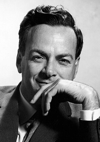
Richard P. Feynman
Richard P. Feynman 1918–1988
🏆 Nobel Física 1965Nobel Physics 1965 🌐 Wikipedia ↗
QM Block IV & V (Ch. 16 & 18) • Hellmann–Feynman Electrostatic Theorem, Analytical Forces & Adiabatic ConnectionQM Bloco IV & V (Cap. 16 & 18) • Teorema Eletrostático de Hellmann–Feynman, Forças Analíticas e Conexão Adiabática 1935–1939 • Nobel Physics 1965

12. Hans Hellmann (1903–1938) & Richard P. Feynman (1918–1988)

Germany/USSR & USA • Authors of the Quantum Force Theorem ($\partial E/\partial\lambda = \langle\Psi|\partial\hat{H}/\partial\lambda|\Psi\rangle$), Pseudopotentials (ECP) & Path Integrals Alemanha/URSS e EUA • Os Autores do Teorema das Forças Quânticas ($\partial E/\partial\lambda = \langle\Psi|\partial\hat{H}/\partial\lambda|\Psi\rangle$), dos Pseudopotenciais (ECP) e dos Integrais de Caminho

How do we compute the force $\mathbf{F}_A = -\nabla_{\mathbf{R}_A}E$ acting on every atomic nucleus to optimize a molecule's 3D geometry without running dozens of finite-difference single-point calculations? In 1937 at the Karpov Institute in Moscow, anti-fascist German physical chemist Hans Hellmann — author of the world's very first textbook titled Einführung in die Quantenchemie ("Introduction to Quantum Chemistry", 1937) and inventor of Effective Core Pseudopotentials (ECP, 1935)! — and independently in 1939 in his undergraduate senior thesis at MIT at age 21, American physicist Richard P. Feynman (1965 Physics Nobel Laureate), proved the remarkable Hellmann–Feynman Theorem: for a variationally stationary wave function, the derivative of the total energy with respect to any parameter $\lambda$ (such as a nuclear coordinate $\mathbf{R}_A$, an external electric field $\mathcal{E}$, or the coupling constant $\lambda \in [0,1]$ in the DFT Adiabatic Connection!) equals the expectation value of the derivative of the Hamiltonian operator alone: $\frac{\partial E}{\partial\lambda} = \langle\Psi|\frac{\partial\hat{H}}{\partial\lambda}|\Psi\rangle$! (When atom-centered basis functions move with the nuclei, Péter Pulay showed in 1969 that adding the basis-set derivative yields the exact analytical Pulay Force!). Como calcular a força $\mathbf{F}_A = -\nabla_{\mathbf{R}_A}E$ que atua sobre cada núcleo atómico para otimizar a geometria 3D de uma molécula sem ter de repetir dezenas de cálculos de energia ponto a ponto? Em 1937, no Instituto Karpov em Moscovo, o físico-químico alemão antifascista Hans Hellmann — autor do primeiro livro de texto do mundo intitulado Einführung in die Quantenchemie («Introdução à Química Quântica», 1937) e inventor dos Pseudopotenciais de Caroço Efetivo (ECP, 1935)! — e, independentemente em 1939 na sua tese de licenciatura no MIT aos 21 anos, o físico americano Richard P. Feynman (Nobel da Física de 1965), demonstraram o extraordinário Teorema de Hellmann–Feynman: para uma função de onda variacionalmente estacionária, a derivada da energia em ordem a qualquer parâmetro $\lambda$ (como uma coordenada nuclear $\mathbf{R}_A$, um campo elétrico externo $\mathcal{E}$ ou o parâmetro de acoplamento $\lambda \in [0,1]$ da Conexão Adiabática em DFT!) é simplesmente o valor esperado da derivada do operador Hamiltoniano: $\frac{\partial E}{\partial\lambda} = \langle\Psi|\frac{\partial\hat{H}}{\partial\lambda}|\Psi\rangle$! (Quando usamos conjuntos de base centrados nos átomos que se movem com os núcleos, Péter Pulay mostrou em 1969 que basta somar a este termo a Força de Pulay da derivada da base!).

SIGNATURE EQUATIONSEQUAÇÕES IMORTAIS ASSOCIADAS $$\frac{\partial E(\lambda)}{\partial \lambda} = \left\langle \Psi(\lambda) \left| \frac{\partial \hat{H}(\lambda)}{\partial \lambda} \right| \Psi(\lambda) \right\rangle, \qquad \mathbf{F}_A^{\text{HF}} = Z_A\int \rho(\mathbf{r})\frac{\mathbf{r}-\mathbf{R}_A}{|\mathbf{r}-\mathbf{R}_A|^3}\,d\mathbf{r} - Z_A\sum_{B\ne A}Z_B\frac{\mathbf{R}_A-\mathbf{R}_B}{|\mathbf{R}_A-\mathbf{R}_B|^3}$$
⚛️ Why They Matter in Quantum & Computational ChemistryPorque são importantes em Química Quântica e Computacional

The Hellmann–Feynman Theorem carries a breathtaking physical message (Ch. 18): once the quantum electron density $\rho(\mathbf{r})$ has been determined by Schrödinger's equation, the force on every atomic nucleus is 100% classical electrostatics (pure Coulomb attraction/repulsion between nuclei and the cloud $\rho(\mathbf{r})$!). Moreover, applying Hellmann–Feynman to the coupling parameter $\lambda \in [0,1]$ yields both the Adiabatic Connection Formula in DFT ($E_{\text{XC}}[\rho] = \int_0^1 \langle\Psi_\lambda|\hat{V}_{ee}|\Psi_\lambda\rangle d\lambda - J[\rho]$, Ch. 16) and Kirkwood's Thermodynamic Integration ($\Delta G = \int_0^1 \langle\partial H/\partial\lambda\rangle_\lambda d\lambda$) in Free-Energy simulations! O Teorema de Hellmann–Feynman tem um significado físico deslumbrante (Cap. 18): uma vez conhecida a densidade eletrónica quântica $\rho(\mathbf{r})$ pela equação de Schrödinger, a força sobre cada núcleo atómico é 100% eletrostática clássica (Lei de Coulomb pura entre os núcleos e a nuvem $\rho(\mathbf{r})$!). Além disso, é o Teorema de Hellmann–Feynman aplicado ao parâmetro $\lambda \in [0,1]$ que permite deduzir a Fórmula da Conexão Adiabática de Harris–Jones–Gunnarsson–Lundqvist ($E_{\text{XC}}[\rho] = \int_0^1 \langle\Psi_\lambda|\hat{V}_{ee}|\Psi_\lambda\rangle d\lambda - J[\rho]$) no Capítulo 16, e exatamente o mesmo teorema aplicado à mecânica estatística que origina a Integração Termodinâmica de Kirkwood ($\Delta G = \int_0^1 \langle\partial H/\partial\lambda\rangle_\lambda d\lambda$)!

🌍 Why They Matter to the World!Porque são importantes para o Mundo!

Feynman's Path Integrals ($Z = \oint \mathcal{D}[\mathbf{r}(\tau)]\,e^{-S_{\text{E}}/\hbar}$) also form the foundation of modern Path-Integral Molecular Dynamics (PIMD / Ring-Polymer MD), which maps quantum nuclei onto ring polymers of classical beads to simulate nuclear quantum tunnelling in enzymes! Os Integrais de Caminho de Feynman ($Z = \oint \mathcal{D}[\mathbf{r}(\tau)]\,e^{-S_{\text{E}}/\hbar}$) são também a base das simulações modernas de Dinâmica Molecular de Integral de Caminho (PIMD / Ring-Polymer MD) que tratam os núcleos atómicos como colares quânticos de contas para simular o efeito de túnel nuclear em enzimas!

😄 Funny Version That You Would Never Forget! 😄A Versão Jocosa que Nunca Mais Vais Esquecer! 😄

Richard Feynman derived the Hellmann–Feynman theorem as a 21-year-old undergraduate at MIT (1939) after his advisor John C. Slater asked him to show how hard it was to calculate forces in molecules — and Feynman came back the next week with a 4-line proof showing it was easy! Feynman later became legendary for playing bongo drums, cracking safes at Los Alamos to expose weak security, and demonstrating the cause of the Space Shuttle Challenger disaster on live television using a simple glass of ice water! Richard Feynman deduziu o Teorema de Hellmann–Feynman quando era ainda um simples aluno de licenciatura de 21 anos no MIT (1939) porque o seu orientador John C. Slater lhe pediu para provar que calcular forças em moléculas era difícil — e Feynman voltou na semana seguinte com uma demonstração de 4 linhas a provar que era simples! Mais tarde, Feynman tornou-se famoso por tocar bongós, arrombar cofres em Los Alamos por diversão para mostrar que os cadeados militares eram inseguros, e explicar em direto na televisão com um copo de água gelada a causa do acidente do vaivém espacial Challenger!

Robert B. Woodward
Robert B. Woodward 1917–1979
🏆 Nobel Química 1965Nobel Chemistry 1965 🌐 Wikipedia ↗
Roald Hoffmann
Roald Hoffmann n. 1937
🏆 Nobel Química 1981Nobel Chemistry 1981 🌐 Wikipedia ↗
Kenichi Fukui
Kenichi Fukui 1918–1998
🏆 Nobel Química 1981Nobel Chemistry 1981 🌐 Wikipedia ↗
QM Block III, IV & V (Ch. 12, 17 & 19) • Frontier Orbitals (HOMO/LUMO) & Orbital SymmetryQM Bloco III, IV & V (Cap. 12, 17 & 19) • Orbitais de Fronteira (HOMO/LUMO) e Simetria Orbital Nobel Chemistry 1965 & 1981

13. Robert B. Woodward (1917–1979), Roald Hoffmann (b. 1937) & Kenichi Fukui (1918–1998)

USA & Japan • Creators of Frontier Molecular Orbital Theory (HOMO/LUMO), the Fukui Function $f(\mathbf{r})$ & the Woodward–Hoffmann Rules EUA e Japão • Os Criadores da Teoria das Orbitais Moleculares de Fronteira (HOMO/LUMO), da Função de Fukui $f(\mathbf{r})$ e das Regras de Woodward–Hoffmann

How can you predict, just by inspecting a molecule's orbitals, which atom a nucleophile or electrophile will attack, and why the Diels–Alder ($[4+2]$) reaction proceeds effortlessly upon heating whereas the $[2+2]$ cycloaddition of two alkenes requires ultraviolet light ($h\nu$)? In 1952 at Kyoto University, Japanese chemist Kenichi Fukui discovered that chemical reactivity is governed by the interaction between the Highest Occupied Molecular Orbital (HOMO, electron donor) of one reactant and the Lowest Unoccupied Molecular Orbital (LUMO, electron acceptor) of the other, defining Frontier Orbital Theory and the Fukui Function $f(\mathbf{r}) = (\partial\rho(\mathbf{r})/\partial N)_v$! In 1965 at Harvard, during the total synthesis of Vitamin $\text{B}_{12}$, legendary synthetic chemist Robert Burns Woodward (1965 Chemistry Nobel Laureate) and young theoretical chemist Roald Hoffmann (creator of Extended Hückel Theory, EHT) formulated the Woodward–Hoffmann Rules of Conservation of Orbital Symmetry: a concerted pericyclic reaction is thermally allowed if and only if the algebraic phase ($+$ vs. $-$) of the occupied molecular orbitals maintains constructive overlap along the entire reaction pathway! Hoffmann and Fukui shared the 1981 Nobel Prize in Chemistry (had Woodward not passed away in 1979, he would have received his second Chemistry Nobel!). Como prever, olhando apenas para as orbitais de uma molécula, em que átomo vai atacar um nucleófilo ou um eletrófilo, e porque é que a reação de Diels–Alder ($[4+2]$) ocorre facilmente por aquecimento enquanto a cicloadição $[2+2]$ de dois alcenos só ocorre com luz ultravioleta ($h\nu$)? Em 1952, na Universidade de Quioto, o químico japonês Kenichi Fukui descobriu que a reatividade química é dominada pela interação entre a Orbital Molecular Ocupada de Maior Energia (HOMO, dadora de eletrões) de um reagente e a Orbital Molecular Desocupada de Menor Energia (LUMO, aceitadora de eletrões) do outro, definindo os Índices de Reatividade de Fronteira e a Função de Fukui $f(\mathbf{r}) = (\partial\rho(\mathbf{r})/\partial N)_v$! Em 1965, em Harvard, durante a síntese total da Vitamina $\text{B}_{12}$, o lendário químico orgânico Robert Burns Woodward (Nobel da Química de 1965) e o jovem químico teórico Roald Hoffmann (criador do método de Hückel Estendido, EHT) descobriram as Regras de Woodward–Hoffmann da Conservação da Simetria Orbital: uma reação pericíclica concertada só é termicamente permitida se a fase algébrica ($+$ vs. $-$) das orbitais moleculares ocupadas se mantiver em interferência construtiva ao longo de toda a coordenada de reação! Hoffmann e Fukui partilharam o Prémio Nobel da Química de 1981 (Woodward tinha falecido em 1979, caso contrário teria ganho o seu segundo Nobel da Química!).

SIGNATURE EQUATIONSEQUAÇÕES IMORTAIS ASSOCIADAS $$\Delta E_{\text{pert}} \approx -\frac{2|\langle \psi_{\text{HOMO}} | \hat{H}' | \psi_{\text{LUMO}} \rangle|^2}{\varepsilon_{\text{LUMO}} - \varepsilon_{\text{HOMO}}}, \qquad f^+(\mathbf{r}) = \rho_{N+1}(\mathbf{r}) - \rho_N(\mathbf{r}) \approx |\psi_{\text{LUMO}}(\mathbf{r})|^2, \qquad f^-(\mathbf{r}) \approx |\psi_{\text{HOMO}}(\mathbf{r})|^2$$
⚛️ Why They Matter in Quantum & Computational ChemistryPorque são importantes em Química Quântica e Computacional

The Woodward–Hoffmann Rules and Fukui's Frontier Orbitals provided the ultimate proof that the algebraic phase sign $+$ and $-$ of the wave function $\psi(\mathbf{r})$ (not just the density $|\psi|^2$!) governs real wet-lab chemistry: where two lobes of the same sign meet, constructive interference forms a bond; where a $+$ lobe meets a $-$ lobe, an antibonding nodal plane creates a prohibitive barrier! As Regras de Woodward–Hoffmann e as Orbitais de Fronteira de Fukui foram a prova definitiva de que o sinal algébrico $+$ e $-$ da função de onda $\psi(\mathbf{r})$ (e não apenas a densidade $|\psi|^2$!) governa a química real na bancada: onde dois lóbulos do mesmo sinal se encontram há interferência construtiva e formação de ligação; onde um lóbulo $+$ encontra um lóbulo $-$ forma-se um plano nodal antiligante e uma barreira proibitiva!

🌍 Why They Matter to the World!Porque são importantes para o Mundo!

Guide the daily design of total syntheses of complex pharmaceuticals, photopharmacology agents, organometallic catalysts, and functional polymers. Guiam diariamente o desenho de sínteses totais de medicamentos complexos, fotofármacos, catalisadores organometálicos e polímeros funcionais.

😄 Funny Version That You Would Never Forget! 😄A Versão Jocosa que Nunca Mais Vais Esquecer! 😄

When Kenichi Fukui published his 1952 paper on "Frontier Orbitals" in the Journal of Chemical Physics, Western chemists initially scoffed at the idea that just 2 electrons in the HOMO could dictate the reactivity of a molecule with 50 or 100 electrons! And Robert B. Woodward was so obsessed with the color blue — always wearing a blue suit, blue shirt, blue tie, and driving a car custom-painted in "Woodward Blue" — that his Harvard students secretly painted his parking space blue at midnight! Quando Kenichi Fukui publicou o seu artigo de 1952 sobre as «Orbitais de Fronteira» no Journal of Chemical Physics, quase todos os químicos ocidentais acharam absurdo que os 2 eletrões da HOMO pudessem mandar mais na reatividade de uma molécula do que todos os outros 50 ou 100 eletrões juntos! E Robert B. Woodward era tão obcecado pela cor azul — vestia sempre fato azul, camisa azul, gravata azul e conduzia um carro pintado à medida no mesmo tom «Azul Woodward» — que os seus alunos de Harvard pintaram secretamente o lugar de estacionamento dele de azul à meia-noite!

Richard F. W. Bader
Richard F. W. Bader 1931–2012
🏆 Criador do QTAIMCreator of QTAIM 🌐 Wikipedia ↗
Maria Goeppert-Mayer
Maria Goeppert-Mayer 1906–1972
🏆 Nobel Física 1963Nobel Physics 1963 🌐 Wikipedia ↗
QM Block V (Ch. 19 & 20) • Quantum Topology QTAIM ($\nabla\rho = \mathbf{0}$) & Two-Photon Nonlinear Spectroscopy (GM)QM Bloco V (Cap. 19 & 20) • Topologia Quântica QTAIM ($\nabla\rho = \mathbf{0}$) e Espetroscopia Não-Linear de Dois Fotões (GM) 1931–1990 • Nobel Physics 1963

14. Richard F. W. Bader (1931–2012) & Maria Goeppert-Mayer (1906–1972)

Canada & Germany/USA • Creator of the Quantum Theory of Atoms in Molecules (QTAIM) & Pioneer of Two-Photon Absorption and Spin–Orbit Coupling Canadá e Alemanha/EUA • O Criador da Teoria Quântica de Átomos em Moléculas (QTAIM) e a Pioneira da Absorção de Dois Fotões e do Acoplamento Spin–Órbita

Where does one atom end and its neighbor begin inside a molecule, and how can we define a chemical bond purely from physical observables without arbitrary basis-set partitioning? At McMaster University (Canada), Richard F. W. Bader created the Quantum Theory of Atoms in Molecules (QTAIM): analyzing the gradient vector field of the observable electron density $\nabla\rho(\mathbf{r})$ (measurable both computationally and by high-resolution X-ray diffraction!), Bader proved that each atom in a molecule is a spatial basin $\Omega_A$ bounded by a zero-flux surface ($\nabla\rho(\mathbf{r})\cdot\mathbf{n}(\mathbf{r}) = 0$) satisfying the quantum virial theorem ($2T_A + V_A = 0$), and that every chemical bond traces a ridge of maximum density containing a Bond Critical Point (BCP, $(3,-1)$, where $\nabla\rho(\mathbf{r}_c)=\mathbf{0}$) whose Laplacian $\nabla^2\rho(\mathbf{r}_c)$ distinguishes shared covalent bonds ($\nabla^2\rho \lt 0$) from closed-shell hydrogen bonds and ionic interactions ($\nabla^2\rho > 0$)! Meanwhile, in Göttingen and the USA, Maria Goeppert-Mayer (Max Born's 1931 PhD student and 1963 Physics Nobel Laureate for the spin–orbit shell model!) derived in her 1931 dissertation the second-order quantum theory of Simultaneous Two-Photon Absorption (TPA) — thirty years before the laser was invented! Onde acaba um átomo e começa o átomo vizinho dentro de uma molécula, e o que é uma ligação química sem depender de escolhas arbitrárias de conjuntos de base? Na Universidade McMaster (Canadá), Richard F. W. Bader criou a Teoria Quântica de Átomos em Moléculas (QTAIM): analisando o campo vetorial do gradiente da densidade eletrónica observável $\nabla\rho(\mathbf{r})$ (medida tanto por cálculos quânticos como por difração de raios X de alta resolução!), Bader provou que cada átomo numa molécula é uma bacia espacial $\Omega_A$ delimitada por uma superfície de fluxo zero ($\nabla\rho(\mathbf{r})\cdot\mathbf{n}(\mathbf{r}) = 0$) onde o Teorema Virial Quântico ($2T_A + V_A = 0$) se cumpre individualmente para cada átomo, e que cada ligação química corresponde a um caminho de densidade máxima com um Ponto Crítico de Ligação (BCP, $(3,-1)$, onde $\nabla\rho(\mathbf{r}_c)=\mathbf{0}$) cujo Laplaciano $\nabla^2\rho(\mathbf{r}_c)$ distingue ligações covalentes partilhadas ($\nabla^2\rho \lt 0$) de interações não-covalentes e pontes de hidrogénio ($\nabla^2\rho > 0$)! E em Göttingen e nos EUA, Maria Goeppert-Mayer (aluna de doutoramento de Max Born em 1931 e Prémio Nobel da Física de 1963 pelo modelo de camadas com acoplamento spin–órbita!) deduziu na sua tese de 1931 a teoria quântica de 2.ª ordem da Absorção Simultânea de Dois Fotões (TPA) — trinta anos antes da invenção do laser!

SIGNATURE EQUATIONSEQUAÇÕES IMORTAIS ASSOCIADAS $$\nabla\rho(\mathbf{r})\cdot\mathbf{n}(\mathbf{r}) = 0\;\;(\forall \mathbf{r}\in \partial\Omega_A), \qquad q_A^{\text{QTAIM}} = Z_A - \int_{\Omega_A}\rho(\mathbf{r})\,d\mathbf{r}, \qquad 1\text{ GM} = 10^{-50}\text{ cm}^4\cdot\text{s}\cdot\text{photon}^{-1}$$
⚛️ Why They Matter in Quantum & Computational ChemistryPorque são importantes em Química Quântica e Computacional

In Chapters 19 and 20 we apply both breakthroughs: Bader's QTAIM topology (and its NCI — Non-Covalent Interactions extension based on the reduced density gradient $s(\mathbf{r})$!) is the gold standard for characterizing hydrogen bonds, halogen bonds, and metal–ligand coordination in enzyme active sites; and the unit of two-photon absorption cross-section in TDDFT calculations (Ch. 17 & 20) is named $1\text{ GM}$ (Goeppert-Mayer) in her honor! No Capítulo 19 e no Capítulo 20 estudamos ambos os contributos: a análise topológica QTAIM de Bader (e a sua extensão NCI — Non-Covalent Interactions baseada no gradiente reduzido $s(\mathbf{r})$!) é hoje o padrão ouro para quantificar pontes de hidrogénio, ligações de halogéneo e coordenação metal–ligando em centros ativos enzimáticos; e a unidade de secção eficaz de absorção de dois fotões em TDDFT (Cap. 17 & 20) chama-se universalmente $1\text{ GM}$ (Goeppert-Mayer) em sua honra!

🌍 Why They Matter to the World!Porque são importantes para o Mundo!

Maria Goeppert-Mayer's two-photon fluorescence microscopy today allows neuroscientists to image living neurons firing deep inside intact brain tissue using harmless near-infrared light! A microscopia de fluorescência de dois fotões de Maria Goeppert-Mayer permite hoje observar neurónios vivos a disparar em profundidade dentro do cérebro intacto com luz infravermelha não lesiva!

😄 Funny Version That You Would Never Forget! 😄A Versão Jocosa que Nunca Mais Vais Esquecer! 😄

Eugene Wigner described Maria Goeppert-Mayer's 1931 PhD thesis on two-photon absorption as «a classic reference of clarity and concreteness», yet at the time it seemed impossible to test experimentally because no lamp on Earth was bright enough to deliver two photons to the same molecule simultaneously! Only in 1961, thirty years later, right after the invention of the laser, did physicists observe the exact effect she had predicted — and two years later she won the Nobel Prize! Eugene Wigner descreveu a tese de doutoramento de Maria Goeppert-Mayer de 1931 sobre absorção de dois fotões como «uma referência clássica de clareza e perfeição», mas na altura parecia completamente impossível de testar porque nenhuma lâmpada do mundo conseguia pôr dois fotões no mesmo cromóforo ao mesmo tempo! Só em 1961, trinta anos depois, quando foi inventado o primeiro laser, é que os físicos observaram exatamente o efeito previsto por Goeppert-Mayer — e dois anos mais tarde ela ganhou o Prémio Nobel!

Henry Eyring
Henry Eyring 1901–1981
🏆 Medalha Nacional & Wolf 1980Wolf Prize in Chemistry 1980 🌐 Wikipedia ↗
Michael Polanyi
Michael Polanyi 1891–1976
🏆 Co-Criador da PES & TSTCo-Creator of PES & TST 🌐 Wikipedia ↗
Eugene P. Wigner
Eugene P. Wigner 1902–1995
🏆 Nobel Física 1963Nobel Physics 1963 🌐 Wikipedia ↗
Rudolph A. Marcus
Rudolph A. Marcus n. 1923
🏆 Nobel Química 1992Nobel Chemistry 1992 🌐 Wikipedia ↗
QM Block II & V (Ch. 5, 18 & 21) • Transition-State Theory ($\Delta G^\ddagger$), Wigner Tunnelling & Marcus TheoryQM Bloco II & V (Cap. 5, 18 & 21) • Teoria do Estado de Transição ($\Delta G^\ddagger$), Túnel de Wigner e Teoria de Marcus 1931–1956 • Nobel Physics 1963 & Chemistry 1992

15. Henry Eyring, Michael Polanyi, Eugene P. Wigner & Rudolph A. Marcus

Mexico/USA, Hungary/UK & Canada/USA • The Four Masters of Activation Barriers ($\Delta G^\ddagger$), Kinetic Tunnelling ($\kappa_{\text{Wigner}}$) & Electron Transfer ($\lambda$) México/EUA, Hungria/Reino Unido e Canadá/EUA • Os Quatro Mestres das Barreiras de Ativação ($\Delta G^\ddagger$), do Efeito de Túnel Cinético ($\kappa_{\text{Wigner}}$) e da Transferência Eletrónica ($\lambda$)

In 1931 in Berlin, Henry Eyring and Michael Polanyi (joined by Eugene Wigner) constructed and plotted the very first reactive Potential Energy Surface in history ($\text{H} + \text{H}_2 \to [\text{H}\cdots\text{H}\cdots\text{H}]^\ddagger \to \text{H}_2 + \text{H}$ — the exact benchmark reaction we compute across 9 functionals in ORCA 5.0.3 in Chapter 16!). Four years later (1935), Henry Eyring and Michael Polanyi (with Meredith Evans) independently derived the Eyring Equation of Transition-State Theory (TST), connecting the macroscopic rate constant $k_{\text{cat}}$ of any chemical or enzymatic reaction to the Gibbs free energy barrier $\Delta G^\ddagger$ of the first-order saddle point ($\nu_{\text{imag}}^\ddagger = i|\nu^\ddagger|$). In 1932, Eugene Wigner (1963 Physics Nobel Laureate for Group Theory and Symmetry in Quantum Mechanics!) derived the Wigner Quantum Tunnelling Correction $\kappa_{\text{Wigner}}(T) = 1 + \frac{1}{24}\left(\frac{h|\nu^\ddagger|}{k_B T}\right)^2$ directly from the magnitude of the transition-state imaginary frequency! And in 1956, Rudolph A. Marcus (1992 Chemistry Nobel Laureate) formulated Marcus Electron Transfer Theory, proving how protein and solvent reorganization energy ($\lambda$) governs biological redox catalysis in photosynthesis and cellular respiration! Em 1931, em Berlim, Henry Eyring e Michael Polanyi (com o auxílio da teoria de grupos de Eugene Wigner) construíram e desenharam a primeira Superfície de Energia Potencial reativa da história ($\text{H} + \text{H}_2 \to [\text{H}\cdots\text{H}\cdots\text{H}]^\ddagger \to \text{H}_2 + \text{H}$ — exatamente a reação que calculamos com 9 funcionais no ORCA 5.0.3 no Capítulo 16!). Quatro anos depois (1935), Henry Eyring e Michael Polanyi (com Meredith Evans) deduziram de forma independente a Equação de Eyring da Teoria do Estado de Transição (TST), ligando a velocidade macroscópica de qualquer reação química ou enzimática ($k_{\text{cat}}$) à barreira de energia livre de Gibbs $\Delta G^\ddagger$ do ponto de sela de 1.ª ordem ($\nu_{\text{imag}}^\ddagger = i|\nu^\ddagger|$). Em 1932, Eugene Wigner (Nobel da Física de 1963 pela aplicação da Teoria de Grupos e Simetria à Mecânica Quântica!) deduziu o Fator de Transmissão de Túnel Quântico de Wigner $\kappa_{\text{Wigner}}(T) = 1 + \frac{1}{24}\left(\frac{h|\nu^\ddagger|}{k_B T}\right)^2$ diretamente a partir do módulo da frequência imaginária do estado de transição! E em 1956, Rudolph A. Marcus (Nobel da Química de 1992) criou a Teoria de Marcus da Transferência Eletrónica, demonstrando como a energia de reorganização eletrostática da proteína e do solvente ($\lambda$) governa a catálise redox na fotossíntese e na respiração celular!

SIGNATURE EQUATIONSEQUAÇÕES IMORTAIS ASSOCIADAS $$k(T) = \kappa(T)\frac{k_B T}{h}\exp\!\left(-\frac{\Delta G^\ddagger}{RT}\right), \qquad \kappa_{\text{Wigner}}(T) = 1 + \frac{1}{24}\left(\frac{h|\nu^\ddagger|}{k_B T}\right)^2, \qquad \Delta G^\ddagger_{\text{Marcus}} = \frac{(\lambda + \Delta G^\circ)^2}{4\lambda}$$
⚛️ Why They Matter in Quantum & Computational ChemistryPorque são importantes em Química Quântica e Computacional

In Chapter 18 (transition states and IRC) and Chapter 21 (RRHO / Quasi-RRHO Statistical Thermochemistry), these three equations convert the numbers printed in an ORCA output file ($\Delta H^\ddagger$, $-T\Delta S^\ddagger$, $\Delta G^\ddagger$, and the imaginary frequency $\nu_{\text{imag}}^\ddagger$) directly into the experimental rate constant $k(T)$ in $\text{s}^{-1}$ and the Kinetic Isotope Effect ($\text{KIE} = k_{\text{H}}/k_{\text{D}}$)! No Capítulo 18 (estados de transição e IRC) e no Capítulo 21 (Termoquímica Estatística RRHO / Quasi-RRHO), estas três equações convertem os números que saem de um ficheiro de output do ORCA ($\Delta H^\ddagger$, $-T\Delta S^\ddagger$, $\Delta G^\ddagger$ e a frequência imaginária $\nu_{\text{imag}}^\ddagger$) na constante de velocidade experimental $k(T)$ em $\text{s}^{-1}$ e no Efeito Isotópico Cinético ($\text{KIE} = k_{\text{H}}/k_{\text{D}}$)!

🌍 Why They Matter to the World!Porque são importantes para o Mundo!

Michael Polanyi's son, John C. Polanyi, went on to win the 1986 Nobel Prize in Chemistry for experimentally observing via infrared chemiluminescence the exact trajectories across Potential Energy Surfaces that his father and Henry Eyring had invented in 1931! O filho de Michael Polanyi, John C. Polanyi, ganhou mais tarde o Prémio Nobel da Química de 1986 por observar experimentalmente por quimioluminescência infravermelha as trajetórias sobre as Superfícies de Energia Potencial que o pai e Henry Eyring tinham inventado em 1931!

😄 Funny Version That You Would Never Forget! 😄A Versão Jocosa que Nunca Mais Vais Esquecer! 😄

Henry Eyring's landmark 1935 Transition-State Theory paper was initially rejected by the Journal of Chemical Physics because a referee thought applying equilibrium partition functions to an unstable saddle point was heresy! And when Rudolph Marcus predicted the "Marcus Inverted Region" in 1960 (making a reaction much more exergonic, $-\Delta G^\circ > \lambda$, actually makes it slower!), skeptics doubted it for 25 years — until Miller, Calcaterra, and Closs experimentally confirmed the inverted parabola in 1984, revealing how green plants prevent charge-recombination short-circuits in photosynthesis! O artigo fundador de Henry Eyring de 1935 sobre a Teoria do Estado de Transição foi inicialmente rejeitado pelo Journal of Chemical Physics porque o revisor achou ridículo aplicar funções de partição de equilíbrio a um complexo ativado que está a desfazer-se no topo da barreira! E quando Rudolph Marcus previu em 1960 a «Região Invertida de Marcus» (tornar uma reação muito mais exergónica, $-\Delta G^\circ > \lambda$, torna a reação mais lenta em vez de mais rápida!), quase ninguém acreditou durante 25 anos — até que em 1984 Miller, Calcaterra e Closs mediram exatamente a parábola invertida de Marcus e demonstraram que é assim que as plantas verdes evitam o curto-circuito na fotossíntese!

Felix Bloch
Felix Bloch 1905–1983
🏆 Nobel Física 1952 (RMN & Sólidos)Nobel Physics 1952 (NMR & Solids) 🌐 Wikipedia ↗
Pekka Pyykkö
Pekka Pyykkö n. 1941
🏆 Química Quântica RelativistaRelativistic Quantum Chemistry 🌐 Wikipedia ↗
QM Block V & VI (Ch. 20 & 22) • Periodic Solids (Bloch's Theorem), NMR & Relativistic Quantum ChemistryQM Bloco V & VI (Cap. 20 & 22) • Sólidos Periódicos (Teorema de Bloch), RMN e Química Quântica Relativista 1928–1979 • Nobel Physics 1952

16. Felix Bloch (1905–1983) & Pekka Pyykkö (b. 1941)

Switzerland/USA & Finland • Creator of Bloch's Theorem for Periodic Crystals & NMR and Pioneer of Heavy-Element Relativistic Quantum Chemistry Suíça/EUA e Finlândia • O Criador do Teorema de Bloch dos Cristais Periódicos e da RMN e o Pioneiro da Química Quântica Relativista dos Elementos Pesados

How can you solve the Schrödinger equation for a catalytic crystal or semiconductor containing $10^{23}$ atoms without an infinite matrix? In 1928, in his Leipzig PhD thesis under Werner Heisenberg, Swiss physicist Felix Bloch proved Bloch's Theorem: in a periodic crystal potential $V(\mathbf{r}+\mathbf{R}_{\mathbf{L}}) = V(\mathbf{r})$, the electronic eigenfunctions are plane waves modulated by a cell-periodic function, $\psi_{n\mathbf{k}}(\mathbf{r}) = e^{i\mathbf{k}\cdot\mathbf{r}}u_{n\mathbf{k}}(\mathbf{r})$, reducing an infinite crystal to a single unit cell in the 1st Brillouin Zone! Eighteen years later (1946) at Stanford, Felix Bloch (simultaneously with Edward Purcell) discovered Nuclear Magnetic Resonance (NMR, 1952 Physics Nobel Prize) and formulated the Bloch Equations of nuclear spin relaxation! And what happens when we move down the Periodic Table to heavy transition metals, lanthanides, and actinides (Ch. 22), where inner $1s$ electrons travel at over $50\%$ of the speed of light ($v/c \approx Z/137$)? Finnish quantum chemist Pekka Pyykkö (University of Helsinki) showed how direct relativistic contraction of $s$ and $p$ orbitals and indirect relativistic expansion and destabilization of $d$ and $f$ orbitals (computed in ORCA via ZORA and DKH2 Hamiltonians!) govern heavy-element chemistry! Como aplicar a equação de Schrödinger a um cristal catalítico ou semicondutor com $10^{23}$ átomos sem ter uma matriz infinita? Em 1928, na sua tese de doutoramento em Leipzig com Werner Heisenberg, o físico suíço Felix Bloch provou o Teorema de Bloch: num potencial cristalino periódico $V(\mathbf{r}+\mathbf{R}_{\mathbf{L}}) = V(\mathbf{r})$, as autofunções eletrónicas são ondas planas moduladas por uma função com a periodicidade da célula unitária, $\psi_{n\mathbf{k}}(\mathbf{r}) = e^{i\mathbf{k}\cdot\mathbf{r}}u_{n\mathbf{k}}(\mathbf{r})$, reduzindo um cristal infinito a uma única célula unitária na 1.ª Zona de Brillouin! Dezoito anos depois (1946), em Stanford, Felix Bloch (em simultâneo com Edward Purcell) descobriu a Ressonância Magnética Nuclear (RMN, Nobel da Física de 1952) e deduziu as Equações de Bloch da magnetização nuclear! E o que acontece quando descemos na Tabela Periódica para os metais de transição pesados, lantanídeos e actinídeos (Cap. 22), onde os eletrões $1s$ se movem a mais de $50\%$ da velocidade da luz ($v/c \approx Z/137$)? O químico quântico finlandês Pekka Pyykkö (Universidade de Helsínquia) revelou como a contração relativista direta das orbitais $s$ e $p$ e a expansão e desestabilização relativista indireta das orbitais $d$ e $f$ (tratadas hoje no ORCA via Hamiltonianos ZORA e DKH2!) governam toda a química dos elementos pesados!

SIGNATURE EQUATIONSEQUAÇÕES IMORTAIS ASSOCIADAS $$\psi_{n\mathbf{k}}(\mathbf{r}) = e^{i\mathbf{k}\cdot\mathbf{r}}\,u_{n\mathbf{k}}(\mathbf{r}) = \frac{1}{\sqrt{\Omega}}\sum_{\mathbf{G}} c_{n,\mathbf{k}+\mathbf{G}}\,e^{i(\mathbf{k}+\mathbf{G})\cdot\mathbf{r}}, \qquad \frac{m_{\text{rel}}}{m_e} = \frac{1}{\sqrt{1 - (Z/137.036)^2}}$$
⚛️ Why They Matter in Quantum & Computational ChemistryPorque são importantes em Química Quântica e Computacional

In Chapter 20 (GIAO NMR Spectroscopy) and Chapter 22 (Periodic Solids, Plane Waves & Relativistic Quantum Chemistry), we see Bloch and Pyykkö's direct impact: without Bloch's Theorem there would be no solid-state DFT codes (VASP, Quantum ESPRESSO, CP2K), and without scalar relativistic Hamiltonians (ZORA/DKH2) we would mispredict bond lengths and catalytic barriers of Gold ($\text{Au}$), Platinum ($\text{Pt}$, such as the anticancer drug Cisplatin!), and Mercury ($\text{Hg}$) complexes by tens of $\text{kcal/mol}$! No Capítulo 20 (Espetroscopia de RMN GIAO) e no Capítulo 22 (Sólidos Periódicos, Ondas Planas e Química Quântica Relativista), vemos o impacto direto de Bloch e Pyykkö: sem o Teorema de Bloch não existiriam códigos de estado sólido (VASP, Quantum ESPRESSO, CP2K), e sem os efeitos relativistas escalares (ZORA/DKH2) erraríamos os comprimentos de ligação e as barreiras catalíticas de complexos de Ouro ($\text{Au}$), Platina ($\text{Pt}$, como o fármaco anticancerígeno Cisplatina!) e Mercúrio ($\text{Hg}$) em dezenas de $\text{kcal/mol}$!

🌍 Why They Matter to the World!Porque são importantes para o Mundo!

Explains three everyday marvels: 1) why Gold ($\text{Au}$, $Z=79$) is yellow rather than silvery like Silver ($\text{Ag}$, $Z=47$); 2) why Mercury ($\text{Hg}$, $Z=80$) is liquid at room temperature; and 3) why cars start in the morning (as Pyykkö proved in 2011, $\sim 1.7\text{ V}$ out of the $2.1\text{ V}$ of every lead-acid car battery cell comes directly from the relativistic contraction of the $6s$ orbital of Lead $\text{Pb}$, $Z=82$!). Explica três maravilhas do quotidiano: 1) porque é que o Ouro ($\text{Au}$, $Z=79$) é dourado e não prateado como a Prata ($\text{Ag}$, $Z=47$); 2) porque é que o Mercúrio ($\text{Hg}$, $Z=80$) é o único metal líquido à temperatura ambiente; e 3) como é que os automóveis arrancam todas as manhãs (segundo Pyykkö, cerca de $1.7\text{ V}$ dos $2.1\text{ V}$ de cada célula de uma bateria de chumbo-ácido vêm diretamente da contração relativista da orbital $6s$ do Chumbo $\text{Pb}$, $Z=82$!).

😄 Funny Version That You Would Never Forget! 😄A Versão Jocosa que Nunca Mais Vais Esquecer! 😄

If Einstein's Special Relativity did not act inside the quantum mechanics of electrons (as demonstrated in Simulator 22.1 of Block VI!), gold wedding rings would look like silvery aluminum foil, mercury thermometers would be solid metal rods at room temperature (non-relativistic mercury melts at $+82^\circ\text{C}$ instead of $-39^\circ\text{C}$!), and no car with a lead-acid battery would ever start in the morning! Se não existisse a Teoria da Relatividade Restrita de Einstein dentro da equação quântica dos eletrões (como nos mostramos no Simulador 22.1 do Bloco VI!), as alianças de casamento de Ouro seriam prateadas como papel de alumínio, os termómetros de Mercúrio seriam barras sólidas (num universo não-relativista o Mercúrio só derreteria a $+82^\circ\text{C}$ em vez de $-39^\circ\text{C}$!) e nenhum carro com bateria de chumbo pegaria de manhã!

🧬 Parte II • Capítulos 17 a 21 (19 Pioneiros com Fotografia)Part II • Chapters 17 to 21 (19 Pioneers with Photographs)

Os Gigantes da Simulação Biomolecular, QM/MM, Energia Livre, Reconhecimento Molecular e Inteligência Artificial The Giants of Biomolecular Simulation, QM/MM, Free Energy, Molecular Recognition & Artificial Intelligence

Como a Mecânica Quântica se uniu à Mecânica Estatística, à Cristalografia de Raios X e às Redes Neuronais Profundas para simular enzimas, prever afinidades de fármacos e resolver o problema do folding proteico. How Quantum Mechanics joined forces with Statistical Mechanics, X-Ray Crystallography, and Deep Neural Networks to simulate enzymes, predict drug binding affinities, and solve the protein folding problem.

Nicholas Metropolis
Nicholas Metropolis 1915–1999
🏆 Algoritmo de MetropolisMetropolis Algorithm 🌐 Wikipedia ↗
Arianna W. Rosenbluth
Arianna W. Rosenbluth 1927–2020
🏆 1.º Código MCMC (1953)1st MCMC Code (1953) 🌐 Wikipedia ↗
Stanislaw Ulam
Stanislaw Ulam 1909–1984
🏆 Co-Inventor Monte CarloCo-Inventor Monte Carlo 🌐 Wikipedia ↗
Edward Teller
Edward Teller 1908–2003
🏆 Jahn–Teller & BET & MCJahn–Teller & BET & MC 🌐 Wikipedia ↗
Berni J. Alder
Berni J. Alder 1925–2020
🏆 Pai da Dinâmica MolecularFather of Molecular Dynamics 🌐 Wikipedia ↗
MD Ch. 2 • Birth of Markov-Chain Monte Carlo (1953) & Molecular Dynamics (1957)MD Cap. 2 • Nascimento do Método de Monte Carlo (1953) e da Dinâmica Molecular (1957) 1946 – 1967 • National Medal of Science

17. Nicholas Metropolis, Arianna W. Rosenbluth, Stanislaw Ulam, Edward Teller & Berni J. Alder

USA & Poland/Hungary • Inventors of Boltzmann Markov-Chain Monte Carlo Sampling & the First Molecular Dynamics Simulations EUA e Polónia/Hungria • Os Inventores da Amostragem de Boltzmann de Monte Carlo e das Primeiras Simulações de Dinâmica Molecular

Between 1946 and 1953 at Los Alamos, Stanislaw Ulam, Nicholas Metropolis, Arianna W. Rosenbluth, Marshall Rosenbluth, Augusta Teller, and Edward Teller (also co-discoverer of the quantum Jahn–Teller distortion effect in transition-metal complexes and the BET adsorption isotherm!) invented on the MANIAC vacuum-tube computer the Markov-Chain Monte Carlo (MCMC) algorithm ($P_{\text{acc}} = \min[1,\exp(-\Delta U/k_BT)]$) — with Arianna Rosenbluth (who earned her Harvard Physics PhD at age 21!) writing the entire machine-code implementation! Four years later (1957) at Livermore, Berni J. Alder and Thomas Wainwright performed the first Molecular Dynamics (MD) simulation in history, integrating equations of motion for colliding spheres and discovering purely entropic fluid–solid phase transitions (complemented in 1967 by Loup Verlet's time-reversible symplectic integrator)! Entre 1946 e 1953, em Los Alamos, Stanislaw Ulam, Nicholas Metropolis, Arianna W. Rosenbluth, Marshall Rosenbluth, Augusta Teller e Edward Teller (também co-autor do famoso efeito quântico de distorção de Jahn–Teller em complexos de metais de transição e da isotérmica de adsorção BET!) criaram no computador de válvulas MANIAC o algoritmo de Monte Carlo de Cadeia de Markov (MCMC) ($P_{\text{acc}} = \min[1,\exp(-\Delta U/k_BT)]$) — tendo Arianna Rosenbluth (que se doutorou em Física em Harvard aos 21 anos!) escrito sozinha todo o código-máquina da simulação! Quatro anos depois (1957), em Livermore, Berni J. Alder e Thomas Wainwright realizaram a primeira simulação de Dinâmica Molecular (MD) da história, integrando as equações de movimento de partículas em colisão e descobrindo transições de fase sólido–fluido puramente entrópicas (complementada em 1967 pelo integrador simpético reversível no tempo de Loup Verlet)!

SIGNATURE EQUATIONSEQUAÇÕES IMORTAIS ASSOCIADAS $$P_{\text{acc}}(\text{old}\to\text{new}) = \min\!\left(1,\,e^{-\Delta U / k_B T}\right), \qquad \mathbf{r}_i(t+\Delta t) = 2\mathbf{r}_i(t) - \mathbf{r}_i(t-\Delta t) + \frac{\mathbf{F}_i(t)}{m_i}\Delta t^2$$
⚛️ Why They Matter in Quantum & Computational ChemistryPorque são importantes em Química Quântica e Computacional

The Metropolis algorithm and Molecular Dynamics bridge Quantum Mechanics (which supplies potential energy surfaces and force-field parameters) with macroscopic Statistical Thermodynamics ($\langle A\rangle = \int A(\mathbf{R})e^{-\beta U(\mathbf{R})}d\mathbf{R} / Z$). O algoritmo de Metropolis e a Dinâmica Molecular unem a Mecânica Quântica (que fornece as superfícies de energia potencial e parâmetros de campo de forças) à Termodinâmica Estatística macroscópica ($\langle A\rangle = \int A(\mathbf{R})e^{-\beta U(\mathbf{R})}d\mathbf{R} / Z$).

🌍 Why They Matter to the World!Porque são importantes para o Mundo!

The 1953 Metropolis algorithm was named #1 among the "Top 10 Algorithms of the 20th Century," powering computational biophysics, Bayesian inference, machine learning, and statistical physics. O algoritmo de Metropolis de 1953 foi eleito o #1 dos «10 Maiores Algoritmos do Século XX», sustentando a biofísica computacional, a inferência Bayesiana, o treino de redes neuronais e a física estatística.

😄 Funny Version That You Would Never Forget! 😄A Versão Jocosa que Nunca Mais Vais Esquecer! 😄

Why is it called the "Monte Carlo" method? While recovering from illness in the hospital playing solitaire, Stanislaw Ulam tried to compute the probability of winning a solitaire hand combinatorially, gave up, and realized: "It's much easier to just deal 100 random hands and count how many win!" Because Ulam's uncle constantly borrowed money from relatives to gamble at the Monte Carlo Casino in Monaco, Nicholas Metropolis christened the method "Monte Carlo"! Porque é que se chama método de «Monte Carlo»? Porque Stanislaw Ulam estava convalescente no hospital a jogar paciências (solitaire) com cartas, tentou calcular a probabilidade de ganhar um jogo de paciência por análise combinatória, desistiu e pensou: «É muito mais fácil distribuir 100 jogos aleatórios e contar quantos ganho!» Como o tio de Ulam pedia constantemente dinheiro emprestado à família para ir jogar à roleta no Casino de Monte Carlo no Mónaco, Nicholas Metropolis batizou o método como «Monte Carlo»!

Shneior Lifson
Shneior Lifson 1914–2001
🏆 Prémio Israel 1969 (CFF)Israel Prize 1969 (CFF) 🌐 Wikipedia ↗
Martin Karplus
Martin Karplus 1930–2024
🏆 Nobel Química 2013Nobel Chemistry 2013 🌐 Wikipedia ↗
Michael Levitt
Michael Levitt n. 1947
🏆 Nobel Química 2013Nobel Chemistry 2013 🌐 Wikipedia ↗
Arieh Warshel
Arieh Warshel n. 1940
🏆 Nobel Química 2013Nobel Chemistry 2013 🌐 Wikipedia ↗
QM Ch. 21 & MD Ch. 1 • Biomolecular Force Fields, Protein MD & Hybrid QM/MM MethodsQM Cap. 21 & MD Cap. 1 • Campos de Forças Biomoleculares, DM de Proteínas e Métodos Híbridos QM/MM Nobel Prize in Chemistry 2013

18. Shneior Lifson (1914–2001), Martin Karplus (1930–2024), Michael Levitt & Arieh Warshel

Israel, Austria/USA & UK • Creators of Consistent Force Fields (CFF, CHARMM), Protein MD & QM/MM Enzymatic Catalysis Israel, Áustria/EUA e Reino Unido • Os Criadores dos Campos de Forças Consistentes (CFF, CHARMM), da DM de Proteínas e da Catálise Enzimática QM/MM

In the late 1960s at the Weizmann Institute in Rehovot (Israel), Shneior Lifson, together with his PhD student Arieh Warshel and young researcher Michael Levitt, formulated the Consistent Force Field (CFF): expressing the potential energy of any biomolecule as an analytical sum of harmonic bonds, angles, periodic torsions, Lennard-Jones 12-6 van der Waals terms, and Coulomb electrostatics. Joining forces with Martin Karplus at Harvard (author of the quantum-mechanical Karplus Equation for $^3J_{\text{HH}}(\phi)$ vicinal NMR coupling constants in Ch. 20 and founder of CHARMM!), they published the landmark 1976 Warshel & Levitt Hybrid QM/MM paper on lysozyme catalysis and the 1977 McCammon, Gelin & Karplus first-ever Molecular Dynamics simulation of a protein (BPTI), earning Karplus, Levitt, and Warshel the 2013 Nobel Prize in Chemistry! No final dos anos 1960, no Instituto Weizmann em Rehovot (Israel), Shneior Lifson, juntamente com o seu aluno de doutoramento Arieh Warshel e o jovem investigador Michael Levitt, formulou o Campo de Forças Consistente (CFF): exprimir a energia potencial de qualquer biomolécula como uma soma analítica de ligações harmónicas, ângulos, torsões periódicas, van der Waals de Lennard-Jones 12-6 e eletrostática de Coulomb. Em colaboração com Martin Karplus em Harvard (autor da célebre Equação Quântica de Karplus para constantes de acoplamento vicinal $^3J_{\text{HH}}(\phi)$ em RMN no Cap. 20 e fundador do CHARMM!), publicaram o histórico artigo de 1976 de Warshel & Levitt sobre o método híbrido QM/MM (aplicado ao mecanismo catalítico da lisozima!) e a primeira simulação de Dinâmica Molecular de uma proteína em 1977 (McCammon, Gelin & Karplus, BPTI), valendo a Karplus, Levitt e Warshel o Prémio Nobel da Química de 2013!

SIGNATURE EQUATIONSEQUAÇÕES IMORTAIS ASSOCIADAS $$\hat{H}_{\text{QM/MM}}^{\text{EE}} = \hat{H}_{\text{QM}}(\mathbf{r};\mathbf{R}_{\text{QM}}) - \sum_{i\in\text{QM}}\sum_{M\in\text{MM}}\frac{q_M}{|\mathbf{r}_i - \mathbf{R}_M|} + \sum_{A\in\text{QM}}\sum_{M\in\text{MM}}\left(\frac{Z_A q_M}{R_{AM}} + V_{AM}^{\text{LJ}}\right) + V_{\text{MM}}(\mathbf{R}_{\text{MM}})$$
⚛️ Why They Matter in Quantum & Computational ChemistryPorque são importantes em Química Quântica e Computacional

In Chapter 21 (Section 21.4), we study in detail Warshel & Levitt's Electrostatic Embedding QM/MM Hamiltonian: the reactive enzyme active site (where covalent bonds break and form) is treated with Kohn–Sham DFT or DLPNO-CCSD(T), polarized directly by the electric field of the point charges $q_M$ of the surrounding MM protein residues and water! No Capítulo 21 (Secção 21.4), estudamos em detalhe o Hamiltoniano QM/MM com Incorporação Eletrostática (Electrostatic Embedding) de Warshel & Levitt: a região reativa do centro ativo (onde ligações covalentes se quebram e formam) é tratada com DFT de Kohn–Sham ou DLPNO-CCSD(T), polarizada diretamente pelo campo elétrico das cargas pontuais $q_M$ dos milhares de resíduos da proteína e da água MM!

🌍 Why They Matter to the World!Porque são importantes para o Mundo!

As the Royal Swedish Academy of Sciences proclaimed in 2013: «They made Newton's classical physics work side-by-side with fundamentally different quantum physics, taking the chemical experiment into cyberspace!» Como escreveu a Real Academia Sueca das Ciências no anúncio do Nobel de 2013: «Eles casaram a Física Quântica de Schrödinger com a Física Clássica de Newton e levaram a experiência química para o ciberespaço!»

😄 Funny Version That You Would Never Forget! 😄A Versão Jocosa que Nunca Mais Vais Esquecer! 😄

How long was the historic 1977 Nobel-winning first Molecular Dynamics simulation of a protein (BPTI, 58 residues, in vacuum without a single water molecule)? Just $9.2\text{ picoseconds}$ ($0.0092\text{ nanoseconds}$)! Today, a single GPU in the BIA Lab simulates over $300\text{ ns/day}$ of a solvated 50,000-atom enzyme — $32,000$ times longer per day than the simulation that won the Nobel Prize! Qual foi a duração total da histórica primeira simulação de Dinâmica Molecular de uma proteína em 1977 (BPTI, apenas 58 aminoácidos, em vácuo sem uma única molécula de água)? Apenas $9.2\text{ picossegundos}$ ($0.0092\text{ nanossegundos}$)! Hoje, uma única placa gráfica GPU no BIA Lab simula mais de $300\text{ ns/dia}$ de uma enzima solvatada com $50\,000$ átomos — $32\,000$ vezes mais tempo por dia do que a simulação que ganhou o Prémio Nobel!

Michele Parrinello
Michele Parrinello n. 1945
🏆 Medalha Dirac & Prémio DreyfusDirac Medal & Dreyfus Prize 🌐 Wikipedia ↗
Charles H. Bennett
Charles H. Bennett n. 1943
🏆 Prémio Wolf de Física 2018Wolf Prize in Physics 2018 🌐 Wikipedia ↗
QM Ch. 22 & FE Ch. 1–36 • Ab Initio Molecular Dynamics (AIMD), Metadynamics & Free Energy (BAR)QM Cap. 22 & FE Cap. 1–36 • Dinâmica Molecular Ab Initio (AIMD), Metadinâmica e Energia Livre (BAR) 1976 – 2008 • Dirac Medal & Wolf Prize

19. Michele Parrinello (b. 1945) & Charles H. Bennett (b. 1943)

Italy/Switzerland & USA • Creator of Car–Parrinello Ab Initio MD (AIMD), the NPT Barostat & Metadynamics, and Inventor of the BAR Free-Energy Estimator & Quantum Information Itália/Suíça e EUA • O Criador da Dinâmica Molecular Ab Initio de Car–Parrinello (AIMD), do Baróstato NPT e da Metadinâmica, e o Inventor do Estimador BAR e da Computação Quântica

In 1985, Italian physicist Michele Parrinello (together with Roberto Car) revolutionized Quantum Chemistry and Condensed-Matter Physics by inventing Car–Parrinello Ab Initio Molecular Dynamics (CPMD / AIMD, Ch. 22): instead of relying on a pre-parameterized classical force field, nuclear forces at every femtosecond time step are computed on the fly from Kohn–Sham DFT electronic structure by treating the orbitals $\{\psi_i\}$ as dynamical variables with a fictitious mass $\mu$! Parrinello also invented the Parrinello–Rahman Anisotropic Barostat (1981), Metadynamics (2002, with Alessandro Laio), and the Canonical Stochastic Velocity-Rescaling Thermostat (v-rescale, 2007, with Giovanni Bussi and Davide Donadio)! Meanwhile at IBM Research, American chemical physicist Charles H. Bennett — who is simultaneously a founding father of Quantum Information Theory, Quantum Cryptography (BB84), and Quantum Teleportation! — derived in 1976 the Bennett Acceptance Ratio (BAR), the minimum-variance statistically optimal estimator for computing free-energy differences $\Delta G$ between two thermodynamic states! Em 1985, o físico italiano Michele Parrinello (juntamente com Roberto Car) revolucionou a Química Quântica e a Física da Matéria Condensada ao inventar a Dinâmica Molecular Ab Initio de Car–Parrinello (CPMD / AIMD, Cap. 22): em vez de usarem um campo de forças clássico parametrizado, as forças nucleares a cada passo de tempo de femtossegundo são calculadas «on-the-fly» a partir da estrutura eletrónica de DFT de Kohn–Sham, tratando as orbitais eletrónicas $\{\psi_i\}$ como variáveis dinâmicas com uma massa fictícia $\mu$! Além disso, Parrinello criou o Baróstato Anisotrópico de Parrinello–Rahman (1981), a Metadinâmica (2002, com Alessandro Laio) e o Termóstato Estocástico Canónico v-rescale (2007, com Giovanni Bussi e Davide Donadio)! E na IBM Research, o físico-químico americano Charles H. Bennett — que é simultaneamente um dos pais fundadores da Teoria da Informação Quântica, Criptografia Quântica (BB84) e Teleportação Quântica! — deduziu em 1976 o célebre estimador Bennett Acceptance Ratio (BAR), o método estatisticamente ótimo de variância mínima para calcular diferenças de energia livre $\Delta G$ entre dois estados termodinâmicos!

SIGNATURE EQUATIONSEQUAÇÕES IMORTAIS ASSOCIADAS $$\mathcal{L}_{\text{CP}} = \sum_I \frac{1}{2}M_I\dot{\mathbf{R}}_I^2 + \sum_i \frac{1}{2}\mu\langle\dot{\psi}_i|\dot{\psi}_i\rangle - E_{\text{KS}}[\{\psi_i\},\{\mathbf{R}_I\}] + \sum_{ij}\Lambda_{ij}(\langle\psi_i|\psi_j\rangle - \delta_{ij}), \qquad \sum_{n=1}^{N_A}\frac{1}{1 + \frac{N_A}{N_B}e^{\beta(\Delta U_n^A - \Delta G)}} = \sum_{m=1}^{N_B}\frac{1}{1 + \frac{N_B}{N_A}e^{-\beta(\Delta U_m^B - \Delta G)}}$$
⚛️ Why They Matter in Quantum & Computational ChemistryPorque são importantes em Química Quântica e Computacional

Ab Initio Molecular Dynamics (AIMD, Ch. 22) enables parameter-free simulation of chemical reactions in liquid water (such as Grotthuss proton hopping $\text{H}_3\text{O}^+ \to \text{H}_2\text{O}$) and on catalytic surfaces, while Metadynamics and BAR reconstruct complete free-energy landscapes $\Delta G(\xi)$! A Dinâmica Molecular Ab Initio (AIMD, Cap. 22) permite simular reações químicas em água líquida (como o mecanismo de transporte de protões de Grotthuss $\text{H}_3\text{O}^+ \to \text{H}_2\text{O}$) e em superfícies catalíticas sem qualquer parâmetro empírico de ligação, enquanto a Metadinâmica e o BAR permitem reconstruir perfis completos de energia livre $\Delta G(\xi)$!

🌍 Why They Matter to the World!Porque são importantes para o Mundo!

Unites electronic-structure Quantum Chemistry, Free-Energy Statistical Physics, and modern Quantum Information Science. Une a Química Quântica de estrutura eletrónica, a Física Estatística de Energia Livre e a Computação Quântica moderna.

😄 Funny Version That You Would Never Forget! 😄A Versão Jocosa que Nunca Mais Vais Esquecer! 😄

How did Michele Parrinello and Alessandro Laio explain Metadynamics to students in 2002? Picture a hiker who falls at night into an empty swimming pool (a free-energy local minimum) and cannot see the exit: if the hiker dumps a bucket of sand on the floor at every step (a Gaussian bias potential $V_{\text{bias}}$), eventually the pool fills up with sand to the rim, the hiker walks out into the next valley, and the total pile of sand poured in is the exact negative image of the free-energy profile $-\Delta G(\xi)$! Como é que Michele Parrinello e Alessandro Laio explicaram a Metadinâmica aos alunos em 2002? Imagine um alpinista que cai de noite numa piscina vazia (um mínimo local de energia livre) sem conseguir ver a saída: se o alpinista despejar um balde de areia no chão sempre que dá um passo ($V_{\text{bias}}$ Gaussiano), mais cedo ou mais tarde a piscina fica cheia de areia até à borda, o alpinista sai a caminhar para a piscina seguinte, e a quantidade de areia que gastou é exatamente o simétrico do perfil de energia livre $-\Delta G(\xi)$!

Hermann Emil Fischer
Hermann Emil Fischer 1852–1919
🏆 Nobel Química 1902Nobel Chemistry 1902 🌐 Wikipedia ↗
Daniel E. Koshland Jr.
Daniel E. Koshland Jr. 1920–2007
🏆 Modelo Induced-Fit (1958)Induced-Fit Model (1958) 🌐 Wikipedia ↗
Dorothy Crowfoot Hodgkin
Dorothy Crowfoot Hodgkin 1910–1994
🏆 Nobel Química 1964Nobel Chemistry 1964 🌐 Wikipedia ↗
DVS Ch. 1–6 & QM Ch. 19 • Lock-and-Key, Induced-Fit & 3D Biomolecular Electron DensityDVS Cap. 1–6 & QM Cap. 19 • Chave-Fechadura, Encaixe Induzido e Densidade Eletrónica 3D de Biomoléculas Nobel Chemistry 1902 & 1964

20. Hermann Emil Fischer (1852–1919), Daniel E. Koshland Jr. (1920–2007) & Dorothy Crowfoot Hodgkin (1910–1994)

Germany, USA & UK • Creators of Enzyme–Ligand Molecular Recognition Models & 3D Biomolecular X-Ray Electron Density Maps Alemanha, EUA e Reino Unido • Os Criadores dos Modelos de Reconhecimento Molecular Enzima–Ligando e da Cristalografia 3D de Fármacos e Proteínas

Before any Molecular Docking program (DOCK by Tack Kuntz, AutoDock by Arthur Olson, Vina by Oleg Trott, GOLD by Gareth Jones, or GNINA by David Koes) or QM/MM calculation could exist, three scientific pillars were required: in 1894, German chemist Hermann Emil Fischer (1902 Chemistry Nobel Laureate) formulated the "Lock-and-Key" (Schlüssel-Schloss-Prinzip) model of stereochemical and electrostatic complementarity between an enzyme and its substrate. In 1958, American biochemist Daniel E. Koshland Jr. proved that enzyme active sites are not rigid keyholes, formulating the Induced-Fit Theory: ligand binding induces a conformational reorganization of the protein that aligns catalytic residues! And at Oxford, British crystallographer Dorothy Crowfoot Hodgkin (1964 Nobel Prize in Chemistry) pioneered the use of early electronic computers to reconstruct 3D electron density maps $\rho(\mathbf{r})$ from X-ray diffraction, solving the atomic structures of Penicillin (1945), Vitamin $\text{B}_{12}$ (1954, the landmark cobalt corrin cofactor!), and the protein hormone Insulin (1969) — launching Structural Biology and the Protein Data Bank (PDB)! Antes de qualquer programa de Docking Molecular (DOCK de Tack Kuntz, AutoDock de Arthur Olson, Vina de Oleg Trott, GOLD de Gareth Jones ou GNINA de David Koes) ou cálculo QM/MM poder existir, foram necessários três pilares científicos: em 1894, o químico alemão Hermann Emil Fischer (Nobel da Química de 1902) enunciou o modelo «Chave na Fechadura» (Schlüssel-Schloss-Prinzip) da complementaridade estereoquímica e eletrostática entre uma enzima e o seu substrato. Em 1958, o bioquímico americano Daniel E. Koshland Jr. demonstrou que os centros ativos enzimáticos não são fechaduras rígidas, formulando a Teoria do Encaixe Induzido (Induced Fit): a ligação do ligando induz uma reorganização conformacional da proteína que alinha os resíduos catalíticos! E em Oxford, a cristalógrafa britânica Dorothy Crowfoot Hodgkin (Prémio Nobel da Química de 1964) foi pioneira no uso de computadores eletrónicos para reconstruir os mapas tridimensionais da densidade eletrónica $\rho(\mathbf{r})$ por difração de raios X, determinando as estruturas 3D da Penicilina (1945), da Vitamina $\text{B}_{12}$ (1954, o maior complexo bioinorgânico de cobalto!) e da proteína Insulina (1969) — inaugurando a Biologia Estrutural e o Protein Data Bank (PDB)!

SIGNATURE EQUATIONSEQUAÇÕES IMORTAIS ASSOCIADAS $$\rho(\mathbf{r}) = \frac{1}{V_{\text{cell}}}\sum_{hkl} |F_{hkl}|\,e^{i\alpha_{hkl}}\,e^{-2\pi i(hx+ky+lz)}, \qquad \Delta G_{\text{bind}}^{\text{dock}} = \Delta G_{\text{vdW}} + \Delta G_{\text{hbond}} + \Delta G_{\text{elec}} + \Delta G_{\text{desolv}} + \Delta G_{\text{tor}}$$
⚛️ Why They Matter in Quantum & Computational ChemistryPorque são importantes em Química Quântica e Computacional

What an X-ray crystallographer measures in Dorothy Hodgkin's experiment is literally the Fourier transform of the quantum electron density $\rho(\mathbf{r}) = N\int|\Psi|^2 d\tau_{-1}$ studied in Chapters 16 and 19! And the progression from Rigid-Receptor Docking (Fischer's Lock-and-Key) to Flexible-Receptor / Ensemble MD Docking (Koshland's Induced-Fit) is the backbone of Structure-Based Drug Design! O que um cristalógrafo de raios X mede na experiência de Dorothy Hodgkin é literalmente a transformada de Fourier da densidade eletrónica quântica $\rho(\mathbf{r}) = N\int|\Psi|^2 d\tau_{-1}$ estudada nos Capítulos 16 e 19! E a progressão do Docking Rígido (Chave-Fechadura de Fischer) para o Docking Flexível / Ensemble MD (Encaixe Induzido de Koshland) é a espinha dorsal do Desenho de Fármacos Baseado na Estrutura!

🌍 Why They Matter to the World!Porque são importantes para o Mundo!

Dorothy Hodgkin remains Britain's only female Nobel Laureate in the sciences, and her 3D structures of Penicillin and Insulin saved hundreds of millions of lives by enabling rational design of $\beta$-lactam antibiotics and therapeutic insulins! Dorothy Hodgkin continua a ser a única mulher britânica galardoada com um Prémio Nobel das Ciências, e as suas estruturas 3D da Penicilina e da Insulina salvaram centenas de milhões de vidas através do desenho racional de antibióticos $\beta$-lactâmicos e insulinas recombinantes!

😄 Funny Version That You Would Never Forget! 😄A Versão Jocosa que Nunca Mais Vais Esquecer! 😄

When Daniel Koshland submitted his 1958 "Induced-Fit" manuscript, an indignant referee wrote in the rejection letter: «Emil Fischer's Lock-and-Key principle has stood for 64 years; suggesting that an enzyme changes shape to hug its substrate is pure science fiction!» Today, any student who opens two PDB structures of the same enzyme (open apo state vs. closed holo state clasping an inhibitor, such as the flaps of HIV-1 Protease!) sees Koshland's Induced Fit in 3 seconds! Quando Daniel Koshland submeteu o artigo do «Encaixe Induzido» (Induced Fit) em 1958, um revisor furioso escreveu na carta de rejeição: «A ideia Chave-Fechadura de Emil Fischer está nos livros há 64 anos; sugerir que uma enzima muda de forma ao abraçar o substrato é pura ficção científica!» Hoje, qualquer estudante que abra duas estruturas do PDB da mesma enzima (forma apo aberta vs. forma holo fechada sobre o inibidor, como as flaps da Protease do VIH-1!) vê o Encaixe Induzido de Koshland em 3 segundos!

Christian B. Anfinsen
Christian B. Anfinsen 1916–1995
🏆 Nobel Química 1972Nobel Chemistry 1972 🌐 Wikipedia ↗
Sir Demis Hassabis
Sir Demis Hassabis n. 1976
🏆 Nobel Química 2024Nobel Chemistry 2024 🌐 Wikipedia ↗
John M. Jumper
John M. Jumper n. 1985
🏆 Nobel Química 2024Nobel Chemistry 2024 🌐 Wikipedia ↗
David Baker
David Baker n. 1962
🏆 Nobel Química 2024Nobel Chemistry 2024 🌐 Wikipedia ↗
Structural Biology & AI • Thermodynamic Folding Dogma, AlphaFold2/3 & De Novo Design (Rosetta)Biologia Estrutural & IA • Dogma Termodinâmico do Folding, AlphaFold2/3 e Desenho De Novo (Rosetta) Nobel Prize in Chemistry 1972 & 2024

21. Christian B. Anfinsen (1916–1995), Demis Hassabis, John M. Jumper & David Baker

USA & UK • From the Thermodynamic Dogma of Protein Folding (1972) to the AlphaFold & Rosetta AI Revolution (2024 Nobel Prize) EUA e Reino Unido • Do Dogma Termodinâmico do Folding Proteico (1972) à Revolução de Inteligência Artificial AlphaFold e Rosetta (Nobel 2024)

Between 1961 and 1972 at the NIH, American biochemist Christian B. Anfinsen (1972 Nobel Prize in Chemistry) demonstrated using Ribonuclease A the famous Anfinsen Thermodynamic Hypothesis: a protein's 1D amino-acid sequence holds all the physical information required to specify its native 3D structure, which corresponds to the global minimum of Gibbs Free Energy ($G_{\text{native}} = H - TS$) in its physiological environment! For 50 years, predicting that 3D structure from the 1D sequence alone (overcoming Cyrus Levinthal's Paradox of $3^{100}$ conformations!) remained the "Holy Grail" of computational biology. In 2020–2024, Demis Hassabis and John M. Jumper (Google DeepMind, with Jumper trained in protein statistical physics and MD at the University of Chicago!) solved Anfinsen's problem by creating AlphaFold2 and AlphaFold3 using geometric Evoformer attention and all-atom diffusion networks, while David Baker (University of Washington) solved the inverse problem with Rosetta, RoseTTAFold, and RFdiffusion: designing brand-new proteins never seen in Nature to act as custom enzymes, vaccines, and molecular machines — earning Hassabis, Jumper, and Baker the 2024 Nobel Prize in Chemistry! Em 1961–1972, nos NIH, o bioquímico americano Christian B. Anfinsen (Prémio Nobel da Química de 1972) demonstrou com a enzima Ribonuclease A o célebre Dogma Termodinâmico de Anfinsen: a sequência linear de aminoácidos (1D) contém toda a informação física necessária para determinar a estrutura tridimensional nativa (3D) de uma proteína, que corresponde ao mínimo global de Energia Livre de Gibbs ($G_{\text{nativo}} = H - TS$) no meio fisiológico! Durante 50 anos, prever essa estrutura 3D a partir da sequência 1D (superando o Paradoxo de Cyrus Levinthal de $3^{100}$ conformações possíveis!) foi o «Santo Graal» da biologia computacional. Em 2020–2024, Demis Hassabis e John M. Jumper (Google DeepMind, tendo Jumper feito o doutoramento em simulação de proteínas e física estatística na Universidade de Chicago!) resolveram o problema de Anfinsen criando o AlphaFold2 e o AlphaFold3 com redes de atenção geométrica Evoformer e difusão atómica, enquanto David Baker (Universidade de Washington) resolveu o problema inverso com o Rosetta, RoseTTAFold e RFdiffusion: desenhar proteínas totalmente novas que nunca existiram na Natureza para funcionarem como enzimas artificiais, vacinas e biossensores — partilhando os três o Prémio Nobel da Química de 2024!

SIGNATURE EQUATIONSEQUAÇÕES IMORTAIS ASSOCIADAS $$\Delta G_{\text{fold}} = G_{\text{native}}(\mathbf{R}_0) - G_{\text{unfolded}} = \Delta H_{\text{fold}} - T\Delta S_{\text{fold}} < 0, \qquad \text{pLDDT}_i \in [0, 100]\;\;(\text{Alta confiança: } \text{pLDDT} > 90)$$
⚛️ Why They Matter in Quantum & Computational ChemistryPorque são importantes em Química Quântica e Computacional

Completes the grand arc of the BIA Learn platform: the laws of Quantum Mechanics (QM Course) dictate covalent bonding, charges, and intermolecular forces; Molecular Dynamics and Free-Energy Calculations (MD & FE Courses) sample Anfinsen's thermodynamic funnel; and AlphaFold / Rosetta deliver 3D atomic coordinates across 214 million proteins of the Tree of Life! Fecha o arco completo da plataforma BIA Learn: as leis da Mecânica Quântica (Curso QM) ditam as ligações covalentes, cargas e forças intermoleculares; a Dinâmica Molecular e os Cálculos de Energia Livre (Cursos MD & FE) exploram o funil termodinâmico de Anfinsen; e o AlphaFold / Rosetta fornecem as coordenadas atómicas 3D iniciales para mais de 214 milhões de proteínas da Árvore da Vida!

🌍 Why They Matter to the World!Porque são importantes para o Mundo!

Enables researchers worldwide to design novel biologics, plastic-degrading enzymes, synthetic antibodies, and enzyme inhibitors against any human or pathogen target within weeks. Permite hoje desenhar em semanas novos biofármacos, enzimas que degradam plásticos, anticorpos sintéticos e inibidores enzimáticos contra qualquer alvo humano ou patogénico.

😄 Funny Version That You Would Never Forget! 😄A Versão Jocosa que Nunca Mais Vais Esquecer! 😄

Before founding DeepMind and winning the Chemistry Nobel Prize for AlphaFold, teenage chess prodigy Demis Hassabis co-programmed the hit 1994 video game Theme Park at age 17! And David Baker turned the Rosetta energy function into the multiplayer puzzle game Foldit, whose players solved the 3D crystal structure of the Mason-Pfizer monkey virus retroviral protease in just 10 days — a puzzle that had stumped professional crystallographers for 15 years! Antes de fundar a DeepMind e ganhar o Prémio Nobel da Química pelo AlphaFold, Demis Hassabis foi campeão juvenil de xadrez e co-programou aos 17 anos o célebre videojogo Theme Park (1994)! E David Baker transformou a função de energia do Rosetta num jogo online chamado Foldit, onde jogadores sem formação bioquímica resolveram em apenas 10 dias a estrutura 3D da protease retroviral do vírus Mason-Pfizer — um problema que os cristalógrafos não conseguiam resolver há 15 anos!

← 🔥 Ver os Gigantes da TermodinâmicaView the Giants of Thermodynamics
⚛️ Curso de Mecânica Quântica (24 Capítulos)Quantum Mechanics Course (24 Chapters) → 📖 Capítulo 16 Completo (DFT)Full Chapter 16 (DFT) → ⚡ Curso de Dinâmica Molecular & ΔGMD & Free Energy Course →